Download
1 / 15
150 likes | 259 Views
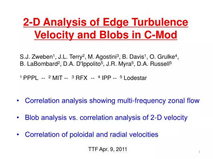
2-D Analysis of Edge Turbulence Velocity and Blobs in C-Mod. S.J. Zweben 1 , J.L. Terry 2 , M. Agostini 3 , B. Davis 1 , O. Grulke 4 , B. LaBombard 2 , D.A. D'Ippolito 5 , J.R. Myra 5 , D.A. Russell 5 1 PPPL -- 2 MIT -- 3 RFX -- 4 IPP -- 5 Lodestar.

E N D
2-D Analysis of Edge Turbulence Velocity and Blobs in C-Mod S.J. Zweben1, J.L. Terry2, M. Agostini3, B. Davis1, O. Grulke4, B. LaBombard2, D.A. D'Ippolito5, J.R. Myra5, D.A. Russell5 1 PPPL -- 2 MIT -- 3 RFX -- 4 IPP -- 5 Lodestar • Correlation analysis showing multi-frequency zonal flow • Blob analysis vs. correlation analysis of 2-D velocity • Correlation of poloidal and radial velocities TTF Apr. 9, 2011
Gas Puff Imaging (GPI) Diagnostic • Optics view along B toward Da emission from D2 gas puff • Oriented to view 2-D radial vs. poloidal plane at gas cloud 2
Alcator C-Mod Gas Puff Imaging • This movie 400,000 frames/sec (normalized to average) • Viewing area ~ 6 cm radially x 6 cm poloidally sep. (EDD) poloidal 3 radial (outward)
What Are We Seeing in GPI ? • Seeing local emission of Da ~ no f(ne,Te)within window where Dais emitted in plasma edge, where Te~ 10 -100 eV • Can measure 2-D turbulence structure and motion even if response of Da is nonlinear (like contrast knob on a TV) • Can not directly measure fluid (ion) flowor ExB flow, but measures turbulence flow velocity, as done previously* * McKee et al, PoP ’03 using BES on DIII-D Conway et al, PPCF ’05 using Doppler reflectometry on AUG 4
Method to Evaluate Turbulence Velocity - for each pixel in each frame, make a short time series of the GPI signal at that pixel over ± 3 frames or 18 µs total - find best match to this time series in pixels of the next frame - find Vrad and Vpol from relative displacement of best match - produces 2-D velocity field with time resolution ~ 40 kHz
Poloidal Velocity vs. Poloidal Position • Estimate ‘zonal flows’ by averaging Vpol over z ~ 5 cm • Typical result has significant poloidal variations of Vpol • Average over these variations to get Vpol(radius, time) one time frame: Vpol vs. z (black) Vpol (ave) red
Poloidally Averaged Velocity vs. Time • Vpol (black) and Vrad (orange) and for r ~ 0 cm • Some cross-correlation between Vpol and Vrad 7
Radial Profiles of Poloidal Velocities • Poloidal velocity fluctuations ~ time-averaged velocities • Implies fluctuating “zonal flow” ~ time-averaged velocity 8
Time Dependence of Velocity Spectra • No clear spectral features lasting more than ~ 1 msec • Looks similar at other radii and for other similar shots 9
Radial Profile of Velocity Spectra • Spectra of Vpol seems to have intermittent harmonic structure • This structure seems localized within ± 1 cm of separatrix 10
Theoretical GAM Frequency for C-Mod • GAM frequency f = G cs/(πR) with G=geometric factor, R = Ro+r, and cs = [(Ti+Te)/mi]1/2 where G~ (2-1/2) (2/(1+k) (1+1/(2A2/3) (1+1/(4q2)) for C-Mod with A=3, k=1.6, q=3, Te=Ti=50 eV, =4/3 and mi=2 fGAM ~ 20 kHz • These analytic values (from R. Hager) can still deviate a factor-of-two from experiment (Hallatschek PPCF 2007)
Blob Analysis of C-Mod GPI Data • Choose threshold for blob detection (e.g. 1.2 x average) • Calculate 2-D velocities from blob trajectories (~ 3 / frame) trajectories of blobs radial profile of blobs
Blob Analysis vs. Correlation Analysis • Choose threshold for blob detection (e.g. 1.2 x average) • Calculate 2-D velocities from blob trajectories (~ 3/frame) • See also Agostini et al (Friday am) for more comparisons poloidal velocity profile radial velocity profile
Correlation of Radial and Poloidal Velocity • Can calculate <dVraddVpol> either zonal-averaged or locally • If RS d/dr<dVraddVpol> = νVpol , then ν ~ 103 sec-1 in SOL local correlations zonal correlations
Summary of 2-D Velocity Analysis • Possible intermittent, multiple-frequency zonal-like flows seen near separatrix in at least some (not all) cases • Velocities from blob-tracking similar to correlation method (both radially outward and in IDD in SOL, as expected) • Correlation between Vrad and Vpol in SOL consistent with Reynolds stress-driven flows assuming ν ~ 103 sec-1 Still very much to learn !