Download
1 / 15
150 likes | 287 Views
Phylogenetic inference on the evolution of protein-coding genes. Lecture 1: Inferences about evolutionary distance Jesse Bloom, jbloom@fhcrc.org. The forward evolutionary process: s (t + dt ) = f [ m { s (t)}]. w ildtype sequence s (t). mutation m(s).

E N D
Phylogenetic inference on the evolution of protein-coding genes Lecture 1: Inferences about evolutionary distance Jesse Bloom, jbloom@fhcrc.org
The forward evolutionary process: s(t + dt) = f[m{s(t)}] wildtype sequence s(t) mutation m(s) selection removes mutation f[m(s)] = s mutation is tolerated and goes to fixation: f[m(s)] = s’
In our homework and on Tuesday, we talked about the forward evolution of the genes. In that case, we imagined that we know the exact mutation and selection processes that were operating. We also imagine that we can see each intermediate produced by evolution. In reality, we do not have access to that information. ggggacatccaa cag ggggacatc cat cag ggggacata cat cag ggcgacata cat cag ggcgacatg cat cag ggcgacatg cataag ggcgacatgcaaaag ggagacatccaacag ggagaaatccaa cag ggagaaatccatcag ggataaatc cat cag gggtaaatc cat cag gggtaaatc catcat
ggggacatccaa cag ggggacatc cat cag ggggacata cat cag ggcgacata cat cag ggcgacatg cat cag ggcgacatg cataag ggcgacatgcaaaag ggagacatccaacag ggagaaatccaa cag ggagaaatccatcag ggataaatc cat cag gggtaaatc cat cag gggtaaatc catcat In this case, an ancestral sequence gave rise to two lineages, each of which experienced six mutations. These led the sequences to differ from the ancestor at 4 and 5 sites, respectively. All we can observe is the final alignment of the sequences, which differ from each other at 7 sites. ggcgacatgcaaaag gggtaaatc catcat
ggggacatccaa cag ggggacatc cat cag ggggacata cat cag ggcgacata cat cag ggcgacatg cat cag ggcgacatg cataag ggcgacatgcaaaag ggagacatccaacag ggagaaatccaa cag ggagaaatccatcag ggataaatc cat cag gggtaaatc cat cag gggtaaatc catcat The question we will ask: how many substitutions have occurred since the divergence of these species. We will call this the “evolutionary distance” in substitution per sites. This will be proportional to time if we assume a molecular clock. ggcgacatgcaaaag gggtaaatc catcat
ggggacatccaa cag ggggacatc cat cag ggggacata cat cag ggcgacata cat cag ggcgacatg cat cag ggcgacatg cataag ggcgacatgcaaaag ggagacatccaacag ggagaaatccaa cag ggagaaatccatcag ggataaatc cat cag gggtaaatc cat cag gggtaaatc catcat The question we will ask: how many substitutions have occurred since the divergence of these species. We will call this the “evolutionary distance” in substitution per sites. This will be proportional to time if we assume a molecular clock. ggcgacatgcaaaag gggtaaatc catcat
We are asking: How long are the branches on this tree? Note that we cannot actually place the root if the substitution model is assumed to be reversible (satisfies detailed balance). But the total summed branch lengths are conserved. ggcgacatgcaaaag gggtaaatc catcat ggcgacatgcaaaag gggtaaatc catcat
Aside: in some very interesting cases, the substitution model is known to be directional (non-reversible)
If we only can see the final sequences, how do we infer the actual number of substitutions that occurred? We must account for reversions and multiple mutations at the same site. ggcgacatgcaaaag gggtaaatc catcat ggcgacatgcaaaag gggtaaatc catcat
At low levels of divergence, the number of substitutions is roughly equal to the Hamming Distance. But at higher levels of divergence, the number of substitutions will be larger than the Hamming Distance. Above is the plot from one of my simulations of the homework.
In order to derive the relationship between sequence identity and number of substitutions, we need a model both for how mutations are distributed among sites in the protein and how the substitutions themselves occur. Recall the simplest model: Jukes-Cantor. Each site mutates with equal probability to any of the other three nucleotides, so a = b = c = d = e = f = μ/3 where μ is the mutation rate. Mutations occur randomly, so the probability of m mutations in time t has mean <m> = μt and the probability of m mutations is: Pr(m | μ, t) = exp(-μt) * (μt)^m / m! Jukes Cantor result: Pr(site is not changed | m mutations) = ¼ + ¾ * exp(-4/3 * m)
More general models of how a sequence can change. The transition matrix. The transition matrix will (in general) be a irreducible and acyclic stochastic matrix. It approaches a unique equilibrium in the limit of long time.
For sites that usually alter protein sequence (such as first and second codon positions), the evolution is clearly dominated by selection on the protein sequence.
We therefore use phenomenological transition matrices that represent both mutation and selection to represent selection on the coding sequence. Let’s look in detail at the WAG matrix…