Download
1 / 41
430 likes | 502 Views
Probing the Sun in 3D Karen Harvey Prize Lecture Boulder 2009. Laurent Gizon Max Planck Institute for Solar System Research, & Goettingen University, Germany. Thanks. Tom Duvall Aaron Birch Sami Solanki. Phil Scherrer.

E N D
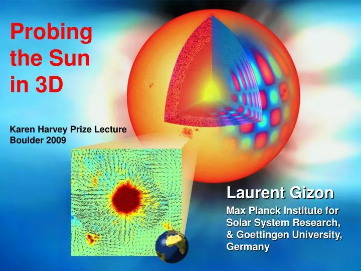
Probing the Sun in 3DKaren Harvey Prize LectureBoulder 2009 Laurent Gizon Max Planck Institute for Solar System Research, & Goettingen University, Germany
Thanks Tom Duvall Aaron Birch Sami Solanki Phil Scherrer This presentation uses material from: Robert Cameron, Jason Jackiewicz, Hannah Schunker
Outline • Helioseismology: Introduction • Why look inside the Sun? • Solar oscillations • Local helioseismology • Probing flows • Probing magnetic activity
Why look inside the Sun? Test the theory of stellar structure and evolution Study effects beyond the standard solar model: Convection, rotation, etc. Everything above the surface is driven by what is happening inside! Why does the Sun have a magnetic field? Solar Dynamo: large-scale flows, 11-yr variations Can we see solar active regions before they emerge at the surface?
Solar oscillations • The Sun is filled with internal acoustic waves with periods near 5 min (freq. near 3 mHz). • Waves are excited by near-surface turbulent convection. • Surface motions (Doppler shifts) are a few 100 m/s, superimposed on the 2 km/s solar rotation. Velocity images (1 min cadence, mean image subtracted) measured with MDI on the SOHO spacecraft
Power spectrum of solar oscillations p modes: pressure waves f modes: surface-gravity waves
Power spectrum of solar oscillations depths < 20 Mm depths < 200 Mm
Global helioseismology • Measurement and inversion of the frequencies of the global modes of resonance (many thousands of individual modes are resolved in freq space) • Among the most precise measurements in astrophysics. • internal structure and rotation as a function of radius and latitude (2D).
Global helioseismology Example: Internal rotation • Frequencies of the normal modes of oscillations are Doppler shifted by rotation • Differential rotation in the convective envelope. • Uniform rotation in the radiative interior. • very small temporal changes connected to the solar cycle red is faster (P=26 days) blue is slower (P=35 days) Schou et al. (1997)
Local helioseismology • A set of techniques to interpret the full wavefield at the solar surface, not just the frequencies of the waves. • The goal is to retrieve 3D vector flows and 3D structural inhomogeneities.
Local Helioseismology T Duvall F Hill C Lindsey M Woodard D Braun
Time-distance helioseismology • A technique to measure the time it takes for waves to propagate between any two point (A,B) on the surface through the interior • Seismic traveltimes contain information about the local properties of the medium . B t- > U . t+ c > A
Time-distance helioseismology • Mean travel times are sensitive to wave-speed perturbations • Differences between the A→B and B→A directions arise from bulk motion along the path. • Travel-time differences are sensitive to flows . B t- > U . t+ c > A
The cross-covariance functionis used to measure the travel times Let us call f the filtered Doppler velocity (a random field). In local helioseismology, a fundamental quantity is the cross-covariance between two surface points A and B: A measure of how fast disturbances travel between A and B Example C(A,B,t) for f modes and a distance A-B of 10 Mm Travel times: t+ for waves to go from A to B t- for waves to go from B to A Flows break the symmetry in t t+
Outline • Helioseismology: Introduction • Probing flows • Meridional circulation • Supergranulation • Depth dependence • Helical flows • Probing magnetic activity
MeridionalFlow Near surface (top ~10 Mm) North-south travel-time differences averaged over longitude ~10 m/s flow from the equator to the poles near the surface Giles (1999) Gizon & Rempel (2008)
MeridionalFlow Solar cycle dependence North-south travel-time differences averaged over longitude 10-15 m/s flow from the equator to the poles near the surface Gizon & Rempel (2008) Gonzalez Hernandez et al. (2008) Giles (1999)
Local travel-time perturbations The annulus / quadrant geometry (Duvall 1997) ingoing – outgoing travel times horizontal divergence of flows T=8.5 hr annulus radius is 12 Mm Each frame is 370 Mm on the side
Convective flows andmotion of small magnetic features Horizontal divergence of flow field at a depth of 1 Mm (30 Mm dominant spatial scale) White shades: Divergent flows Black shades: Convergent flows Red/green: Small magnetic features measured by MDI/SOHO Duvall & Gizon 2000
Lifetime of supergranulation The study of the evolution of supergranulation is made easier (helioseismic maps are almost insensitive to the line of sight projection) Many supergranules persist for a lot longer than 1 day Average Lifetime ~2 days Divergence maps 12 hr averages
Linear inverse problem in time-distance helioseismology Given a set of travel time measurements, Given a reference solar model (horizontally invariant), Given functions (kernels) that give the sensitivity of travel times to small perturbations in the model (e.g. temperature, density, flows), Solve a linear inverse problem to obtain the perturbations in e.g. temperature, density, flows with respect to the model.
horizontal flows Longuest arrow is 500 m/s Arrows: uxand uyat depth 1 Mm
3D vector flows DEPTH (Mm) Jackiewicz, Gizon, Birch (2008)
3D vector flows Note that , which is good! DEPTH (Mm) Jackiewicz, Gizon, Birch (2008)
How deep do velocity structures persist?Coherence of flows (+noise) vs. depth Jackiewicz, Gizon, Birch (2008)
Helical flows: Effect of rotation on convection div = horizontal divergence; curl = vertical component of vorticity Gizon and Duvall (2003)
Outline • Helioseismology: Introduction • Probing flows • Probing magnetic activity • Sunspots
Sunspots How do sunspots form? What is their subsurface structure? Why are sunspots stable? Flows? Do they persist deep in the solar convection zone? What do they tell us about the solar dynamo? Parker
SOHO/MDI Sunspot in AR9787 Doppler Intensity Magnetic field Little evolution over 9 days
Interaction of the solar waves with the sunspot C(t=0 min) C(t=130 min) Cross-covariance between the MDI signal averaged over a vertical line and the MDI signal at any other point in the map. Here for f modes. Gizon 2007; Cameron et al. 2008
Sunspot seismology • A different game: • The effect of B is strong near the surface • We cannot linearize with respect to a quiet-Sun reference solar model • The only possible strategy: • Numerical forward modeling of full waveforms
Numerical Modeling Numerical simulation of wave propagation through a general 3D magnetized solar atmosphere Small amplitude waves: linearized ideal MHD equations (+adhoc wave damping) Initial value problem Spectral in the horizontal coordinates Finite differences in the z direction SLiM, Cameron et al. (2007, 2008)
Background models Solar-like background atmosphere Stabilized against convective instabilities Quiet-Sun atmosphere Sunspot model Monolith Axisymmetric self-similar solution (Deinzer 1965) B0z=3kG
Background models Solar-like background atmosphere Stabilized against convective instabilities Quiet-Sun atmosphere Sunspot model Monolith Axisymmetric self-similar solution (Deinzer 1965) B0z=3kG
Comparison with observations P1 acoustic wave packet
P1 acoustic wave packet Cameron, Schunker, Gizon
Seismology of sunspots: Waves speed up as they go through a sunspot (f, p1-p4) Partial conversion into slow MHD modes extracts energy from the incoming wave packets (Cally & Bogdan) The simple sunspot model that we have tested gives waveforms that are in qualitative agreement with the observations (f and p1-p4) This model sunspot is shallow (<2 Mm) It should be possible to refine the solution by using linear inversions around this simple model.
Points to remember • Helioseismology has produced a considerable amount of discoveries in solar physics: rotation, convection, temporal variations, meridional circulation, etc. • Local helioseismology, although still in development, is playing a key role in revealing the complex interactions between internal flows and the magnetic field. • Probing magnetic activity (and sunspots) is challenging but feasible using numerical simulations of wave propagation. • The fields of helio- and asteroseismology are supported by major space- and ground-based projects.
Future projects/missions • Helioseismology: • Continuation of GONG Network (Since 1995, NSF) • HMI/SDO (2009, NASA): 4k x 4k images, all the time • Solar Orbiter (2017, ESA) • Asteroseismology: • Ground-based telescopes, e.g. VLT • COROT (2007, ESA) • Kepler (2009, NASA) • PLATO (2017, ESA) ? • Ground-based network (SONG)
The Solar Dynamics Observatory (NASA) • Launch: December 2009? • HMI: Doppler velocity for helioseismology + vector B • AIA: multi-wavelength high-cadence imaging of chromosphere/corona • Roughly one 4kx4k image per second, always • Data flow: ~2 TB/day • HMI data: full-disk coverage, all the time, at high spatial resolution: Perfect for local helioseismology and to study the evolution of all active regions from limb to limb!