Chapter 5 Goods and Financial Markets: the IS-LM Model

1. Chapter 5 Goods and Financial Markets: the IS-LM Model Power Point Presentation Brian VanBlarcom Acadia University

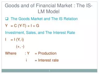
2. THE IS-LM FRAMEWORK The Goods Markets and the IS Relation IS-LM • The IS/LM model is a macroeconomic tool that demonstrates the relationship between interest rates and real output in the goods and services market and the money market. • The intersection of the IS and LM curves is the "General Equilibrium" where there is simultaneous equilibrium in both markets • IS/LM stands for Investment Saving / Liquidity preference Money supply.

3. THE IS-LM FRAMEWORK The Goods Markets and the IS Relation IS-LM - HISTORY • The IS/LM model was born at the Econometric Conference held in Oxford during September, 1936. • Roy Harrod, John R. Hicks, and James Meade all presented papers describing mathematical models attempting to summarize John Maynard Keynes' General Theory of Employment, Interest, and Money.

4. THE IS-LM FRAMEWORK The Goods Markets and the IS Relation IS-LM - HISTORY • Although disputed in some circles and accepted to be imperfect, the model is widely used and seen as useful in gaining an understanding of macroeconomic theory.

5. THE IS-LM FRAMEWORK The Goods Markets and the IS Relation IS-LM - FORMULATION • The model is presented as a graph of two intersecting lines in the first quadrant. • The horizontal axis represents national income or real gross domestic product and is labelled Y. The vertical axis represents the real interest rate, i. Since this is a non-dynamic model, there is a fixed relationship between the nominal interest rate and the real interest rate (the former equals the latter plus the expected inflation rate which is exogenous in the short run); therefore variables such as money demand which actually depend on the nominal interest rate can equivalently be expressed as depending on the real interest rate.

6. THE IS-LM FRAMEWORK The Goods Markets and the IS Relation IS-LM - FORMULATION • The point where these schedules intersect represents a short-run equilibrium in the real and monetary sectors (though not necessarily in other sectors, such as laboUr markets): both the product market and the money market are in equilibrium. This equilibrium yields a unique combination of the interest rate and real GDP. • Lets now begin with our explanation of the IS-LM framework…

7. The Goods Markets and the IS Relation The Goods Markets and the IS Relation The goods market and the IS relation • Equilibrium in the goods market: Production (Y) = Demand (Z) • Demand (Z)= C+I+G C=C(Y-T) T, I, & G are given A Review

8. The Goods Markets and the IS Relation The goods market and the IS relation • Equilibrium: Y=C(Y-T)+I+G • Changes in C, I, & G impact the equilibrium Y A Review (Continued)

9. The Goods Markets and the IS Relation Investment, sales, and the interest rate Investment depends on: The level of sales The interest rate Therefore:

10. Supply of Goods Demand for Goods (Z) The Goods Markets and the IS Relation The IS curve Equilibrium:

11. The Goods Markets and the IS Relation The IS curve ZZ: Demand, a function of Y for given i equilibrium at a, Y ZZ (i) a ZZ´ (i´ > i) Demand, Z b ZZ´: Demand with higher i equilibrium at b, Y´ Y Y´ Output, Y

12. A A´ i´ A´ A i Y´ Y The Goods Markets and the IS Relation The IS curve ZZ (i) Demand, Z ZZ´ (i´ > i) Interest Rate, i IS Y Y´ Output, Y Output, Y

13. The Goods Markets and the IS Relation Observation: In the goods market, the higher the interest rate, the lower the equilibrium output.

14. i IS (T) IS´ (T´ > T) Y Y´ The Goods Markets and the IS Relation The IS curve Shifts in the IS Curve: An increase in taxes shifts the IS curve to the left Interest Rate, i Output, Y

15. i IS´ (G´ > G) IS (G) Y´ Y The Goods Markets and the IS Relation The IS curve Shifts in the IS Curve: An increase in G shifts the IS curve to the right Interest Rate, i Output, Y

16. The Goods Markets and the IS Relation Shifts in the IS curve What do you think: How would a decrease in consumer confidence shift the IS curve?

17. The Financial Market and the LM Relation Money market equilibrium revisited M = nominal money supply (controlled by the Central Bank) $YL(i) = Demand for money (function of nominal income and the interest rate) Equilibrium Interest Rate: M=$YL(i)

18. Real Income Real Money Supply =Real Money Demand: Y(L)i LM relation: The Financial Market and the LM Relation Real money, real income, and the interest rate

19. Ms A´ i´ A i Md´ (for Y´ > Y) Md (for Y) M/P The Financial Market and the LM Relation The LM curve Increase in Y => increases Md which increases i Interest Rate, i (Real) Money, M/P

20. Ms LM (M/P) i´ A´ A´ i´ i A A i Md´ (for Y´ > Y) Md (for Y) M/P Y Y´ The Financial Market and the LM Relation The LM curve Interest Rate, i Interest Rate, i Income, Y (Real) Money, M/P

21. The Financial Market and the LM Relation The LM curve Question: Why does higher economic activity putpressure on interest rates?

22. Ms´ b´ b´ a´ a´ The Financial Market and the LM Relation Shifts in the LM Curve: Showing changes in M & P The LM curve Interest Rate, i LM (M/P) Ms LM´ (M´/P > M/P) i´ b b i´ Interest Rate, i i´2 i´2 a i a i Md´ (for Y´ > Y) i2 i2 Md (for Y) M/P M´/P Y Y´ Income, Y (Real) Money, M/P

23. The IS – LM Model Equilibrium Requires:

24. i & Y is the only interest rate, output combination that yields a simultaneous equilibrium in the goods and financial markets i The IS – LM Model The IS-LM Equilibrium Graphically LM Interest Rate, i IS Y Output, Y

25. A Scenario: The government decides to reduce the budget deficit by increasing taxes, while holding government spending constant. Question: What impact will this fiscal contraction policy have on output and interest rates? Fiscal Policy, Activity and the Interest Rate

26. Fiscal Policy, Activity and the Interest Rate The IS-LM Equilibrium Graphically • IS & LM: Before the tax increase • Equilibrium A: i & Y LM • IS´: After the tax increase • Would the tax increase change • LM? • Disequilibrium at i (F, A) after • tax increase Interest Rate, i A F • i´, Y´ New equilibrium A´ i A´ • The fiscal contraction lowered • interest and output i´ IS (T) IS´ (T´ > T) Y´ Y Output, Y

27. A Scenario: The Bank of Canada engages in monetary expansion, i.e., it increases the money supply through open market operations Question: What impact will the monetary expansion have on output and interest? Monetary Policy, Activity, and the Interest Rate

28. Monetary Policy, Activity, and the Interest Rate The IS-LM Equilibrium Graphically LM (M/P) LM´ (M´/P > M/P) • IS & LM: Before increasing M • Equilibrium A: i & Y Interest Rate, i B • LM´: After increasing M A i • Disequilibrium at i (A, B) A´ i´ • New equilibrium A´: i´ & Y´ • Monetary expansion • lowered i & increased Y IS Y Y´ Output, Y

29. The IS – LM Model The effects of fiscal and monetary policy

30. The policy dilemma of 1993: Record high federal budget deficit (5.4% of GDP) High unemployment and slow growth Deficit reduction reduces output Expansionary fiscal policy increases the deficit Deficit reduction and expansionary monetary policy Recall: Solution: Policy Mix The IS – LM Model The Martin-Thiessen Policy Mix

31. The IS – LM Model The Martin-Thiessen Policy Mix Deficit Reduction and Monetary expansion Insert “In Depth Martin-Thiessen Policy Mix Box from page 91 including text and figure 1

32. The IS – LM Model The Martin-Thiessen Policy Mix Observations: • The combined effect of policies by the government to reduce the deficit and the central bank to lower interest rates allowed the economy to grow significantly from 1994-1999. • This expansion increased tax revenues and helped turn a large deficit into a surplus.

33. The U.S. Economy and the IS-LM Model after 2000

34. The U.S. Economy and the IS-LM Model after 2000

35. The U.S. Economy and the IS-LM Model after 2000 • A review of Figure 4 explains the events around the 2001 recession: • The large shift from IS to IS” represents the decline in investment spending that triggered the recession. • The right shift from LM to LM’ represents the Federal Reserve decision to cut interest rates. • The smaller shift from IS” to IS’ represents the increase in government spending and tax cuts.

36. The U.S. Economy and the IS-LM Model after 2000 • A review of Figure 4 explains the events around the 2001 recession: • The economy would have been at A” without changes in monetary & fiscal policy. • The decline in output was reduced from Y to Y” (without policy changes) to Y to Y’ (with policy changes). • The policy changes made the recession less severe.

37. The U.S. Economy and the IS-LM Model after 2000 Questions • Weren’t the events of September 11, 2001, the cause of the recession? • Why is it not possible to avoid all recessions via monetary and fiscal policy? • Was the monetary-fiscal mix used to fight the recession a textbook example of how policy should be conducted? • Can the recession of 2008, initiated by the very sharp reduction in housing construction, be limited via lower interest rates and tax cuts?

38. LM´ B iB Output decreases slowly B Interest rates adjust instantaneously IS´ Yb Adding Dynamics Dynamics Graphically Goods Market Financial Markets Adjusting to a monetary contraction LM Adjusting to a tax increase Interest Rate, i Interest Rate, i A´ iA iA IS A Ya Ya Output, Y Output, Y

39. Adding Dynamics The Dynamics of Monetary Contraction with IS-LM LM´ LM • A: Initial equilibrium (i & Y) A´´ i´´ Interest Rate, i • LM´: After reducing money • supply A´ i´ • i rises to i´´ A • Higher i reduces demand • and output slowly A´´ to A´ i • New equilibrium at A´: • ( i´, Y´) IS Y´ Y Output, Y

40. Adding Dynamics A Summary • Monetary policy changes interest rates rapidly and output slowly • The Central Bank must consider the output lag when implementing monetary policy

41. Does the IS-LM Model Actually Capture What Happens in the Economy? Does the IS-LM model pass two tests? Are the assumptions of IS-LM reasonable? Are the implications of IS-LM consistent with real-world observations?

42. Does the IS-LM Model Actually Capture What Happens in the Economy? The Empirical Effects of an Increase in the Interest Rates on the Canadian Economy

43. Does the IS-LM Model Actually Capture What Happens in the Economy? The Empirical Effects of an Increase in the Interest Rates on the Canadian Economy

44. Does the IS-LM Model Actually Capture What Happens in the Economy? • The IS-LM model explains movements in economic activity well in the short-run. • The IS-LM model is consistent with economic observations once dynamics are introduced. • An increase in the interest rate due to monetary contraction leads to a steady decline in output. • An increase in investment or consumption leads to an increase in output.

45. Summary • The IS-LM model illustrates the implications in both the goods and financial markets. • The IS relation shows the equilibrium combinations of the interest rate and level of output in the goods market. • An increase in interest rates leads to a decline in output.

46. Summary • The LM relation shows the equilibrium combinations of the interest rate and level of output in the financial markets. • Given the real money supply, an increase in output leads to an increase in the interest rate. • A fiscal expansion shift IS to the right, leading to increased output and interest rate

47. Summary • A monetary expansion shifts the LM curve down, leading to an increase in output and a decrease in interest rates. • The combination of monetary and fiscal policies is know as the policy mix. • Sometimes monetary policy and fiscal policy are used for a common goal.

48. End of Chapter Goods and Financial Markets: the IS-LM Model