Download
1 / 19
190 likes | 201 Views
pTrees p redicate Tree technologie s provide fast, accurate horizontal processing of compressed, data-mining-ready, vertical data structures. 1. 1. 1. 1. 1. 1. 1. 1. 1. 1. 0. 0. course. 2. 3. 4. 5. PINE Podium Incremental Neighborhood Evaluator

E N D
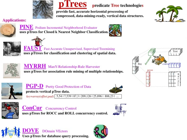
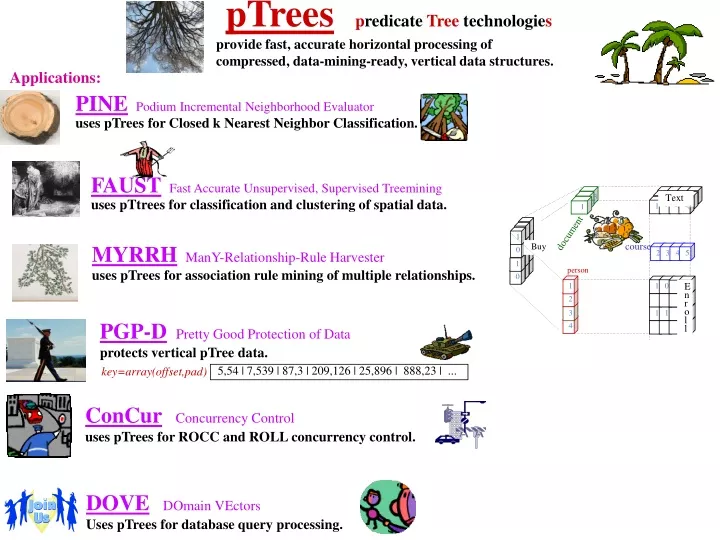
pTreespredicateTreetechnologies provide fast, accurate horizontal processing of compressed, data-mining-ready, vertical data structures. • 1 • 1 • 1 • 1 • 1 • 1 • 1 • 1 1 • 1 • 0 • 0 course 2 3 4 5 PINEPodium Incremental Neighborhood Evaluator uses pTrees for Closed k Nearest Neighbor Classification. 1 0 • 13 Text • 12 1 1 1 • 1 document • 1 1 • 1 • 1 0 Buy • 1 • 1 1 • 1 • 1 person 0 1 Enroll FAUSTFast Accurate Unsupervised, Supervised Treemining uses pTtrees for classification and clustering of spatial data. 2 3 4 MYRRHManY-Relationship-Rule Harvester uses pTrees for association rule mining of multiple relationships. PGP-DPretty Good Protection of Data protects vertical pTree data. key=array(offset,pad) 5,54 | 7,539 | 87,3 | 209,126 | 25,896 | 888,23 | ... ConCurConcurrency Control uses pTrees for ROCC and ROLL concurrency control. DOVEDOmain VEctors Uses pTrees for database query processing. Applications:
pTreespredicateTreetechnologies provide fast, accurate horizontal processing of compressed, data-mining-ready, vertical data structures. predicate Trees (pTrees): project each attribute (now 4 files) 1st, Vertically Processing of Horizontal Data (VPHD) R[A1] R[A2] R[A3] R[A4] R(A1 A2 A3 A4) 2 7 6 1 6 7 6 0 3 7 5 1 2 7 5 7 3 2 1 4 2 2 1 5 7 0 1 4 7 0 1 4 010 111 110 001 011 111 110 000 010 110 101 001 010 111 101 111 011 010 001 100 010 010 001 101 111 000 001 100 111 000 001 100 010 111 110 001 011 111 110 000 010 110 101 001 010 111 101 111 011 010 001 100 010 010 001 101 111 000 001 100 111 000 001 100 for Horizontally structured records, we scan vertically = pure1? true=1 pure1? false=0 R11 R12 R13 R21 R22 R23 R31 R32 R33 R41 R42 R43 0 1 0 1 1 1 1 1 0 0 0 1 0 1 1 1 1 1 1 1 0 0 0 0 0 1 0 1 1 0 1 0 1 0 0 1 0 1 0 1 1 1 1 0 1 1 1 1 0 1 1 0 1 0 0 0 1 1 0 0 0 1 0 0 1 0 0 0 1 1 0 1 1 1 1 0 0 0 0 0 1 1 0 0 1 1 1 0 0 0 0 0 1 1 0 0 pure1? false=0 pure1? false=0 pure1? false=0 0 0 0 1 0 01 0 1 0 1 0 1 1. Whole thing pure1? false 0 P11 P12 P13 P21 P22 P23 P31 P32 P33 P41 P42 P43 2. Left half pure1? false 0 P11 0 0 0 0 0 01 3. Right half pure1? false 0 0 0 0 0 1 0 0 10 01 0 0 0 1 0 0 0 0 0 0 0 1 01 10 0 0 0 0 1 0 0 0 0 1 0 0 0 0 0 0 0 0 0 0 1 0 0 0 0 1 0 0 ^ ^ ^ ^ ^ ^ ^ 0 0 1 0 1 4. Left half of rt half? false0 7 0 1 4 0 0 1 0 0 01 5. Rt half of right half? true1 0 *23 0 0 *22 =2 0 1 *21 *20 0 1 0 To count (7,0,1,4)s use 111000001100P11^P12^P13^P’21^P’22^P’23^P’31^P’32^P33^P41^P’42^P’43 = then vertically slice off each bit position (now 12 files) then compress each bit slice into a pTree e.g., the compression of R11 into P11 goes as follows: =2 e.g., to find the number of occurences of 7 0 1 4 2nd, pTreesfind # of occurences of 7 0 1 4? Base 10 Base 2 R11 0 0 0 0 0 0 1 1 Record the truth of predicate: "pure1 (all 1's)" in a tree recursively on halves, until the half is pure (all 1’s or all 0’s). P11 But it's pure0 so this branch ends
PINEPodium Incremental Neighborhood Evaluator uses pTrees for Closed k Nearest Neighbor Classification (CkNNC) a5 a6a10=Ca11 a12 a13 a14dis from a=000000 area for 3 nearest nbrs C=1 wins! distance=4, don’t replace distance=4, don’t replace distance=2, don’t replace distance=3, don’t replace distance=3, don’t replace distance=2, don’t replace distance=3, don’t replace distance=2, don’t replace distance=2, don’t replace distance=2, don’t replace distance=3, don’t replace distance=2, don’t replace distance=2, don’t replace 0 0 0 0 0 0 0 0 0 0 0 0 0 0 0 0 0 0 0 0 0 0 0 0 0 0 0 0 0 0 0 0 0 0 0 0 0 0 0 0 0 0 0 0 0 0 0 0 0 0 0 0 0 0 0 0 0 0 0 0 0 0 0 0 0 0 0 0 0 0 0 0 0 0 0 0 0 0 distance=1, replace 0 0 0 0 0 0 First 3NN using horizontal data to classify an unclassified sample, a =( 0 0 0 0 0 0 ). t12 0 0 1 0 1 1 0 2 t13 0 0 1 0 1 0 0 1 t53 0 0 0 0 1 0 0 1 t15 0 0 1 0 1 0 1 2 0 1 Key a1 a2 a3 a4a5 a6 a7 a8 a9 a10=Ca11 a12 a13 a14 a15 a16 a17 a18 a19 a20 t12 1 0 1 0 0 0 1 1 0 1 0 1 1 0 1 1 0 0 0 1 t13 1 0 1 0 0 0 1 1 0 1 0 1 0 0 1 0 0 0 1 1 t15 1 0 1 0 0 0 1 1 0 1 0 1 0 1 0 0 1 1 0 0 t16 1 0 1 0 0 0 1 1 0 1 1 0 1 0 1 0 0 0 1 0 t21 0 1 1 0 1 1 0 0 0 1 1 0 1 0 0 0 1 1 0 1 t27 0 1 1 0 1 1 0 0 0 1 0 0 1 1 0 0 1 1 0 0 t31 0 1 0 0 1 0 0 0 1 1 1 0 1 0 0 0 1 1 0 1 t32 0 1 0 0 1 0 0 0 1 1 0 1 1 0 1 1 0 0 0 1 t33 0 1 0 0 1 0 0 0 1 1 0 1 0 0 1 0 0 0 1 1 t35 0 1 0 0 1 0 0 0 1 1 0 1 0 1 0 0 1 1 0 0 t51 0 1 0 1 0 0 1 1 0 0 1 0 1 0 0 0 1 1 0 1 t53 0 1 0 1 0 0 1 1 0 0 0 1 0 0 1 0 0 0 1 1 t55 0 1 0 1 0 0 1 1 0 0 0 1 0 1 0 0 1 1 0 0 t57 0 1 0 1 0 0 1 1 0 0 0 0 1 1 0 0 1 1 0 0 t61 1 0 1 0 1 0 0 0 1 0 1 0 1 0 0 0 1 1 0 1 t72 0 0 1 1 0 0 1 1 0 0 0 1 1 0 1 1 0 0 0 1 t75 0 0 1 1 0 0 1 1 0 0 0 1 0 1 0 0 1 1 0 0
Next C3NN using horizontal data:(a second pass is necessary to find all other voters that are at distance 2 from a) 3NN set after 1st scan Unclassified sample: 0 0 0 0 0 0 a5 a6a10=Ca11 a12 a13 a14distance t12 0 0 1 0 1 1 0 2 t13 0 0 1 0 1 0 0 1 t53 0 0 0 0 1 0 0 1 0 1 d=2, include it also d=2, include it also d=2, include it also d=2, include it also d=4, don’t include d=4, don’t include d=3, don’t include d=3, don’t replace d=3, don’t include d=3, don’t include d=2, include it also d=2, include it also d=2, include it also d=2, include it also 0 0 0 0 0 0 0 0 0 0 0 0 0 0 0 0 0 0 0 0 0 0 0 0 0 0 0 0 0 0 0 0 0 0 0 0 0 0 0 0 0 0 0 0 0 0 0 0 0 0 0 0 0 0 0 0 0 0 0 0 0 0 0 0 0 0 0 0 0 0 0 0 0 0 0 0 0 0 0 0 0 0 0 0 d=1, already voted d=2, already voted d=1, already voted 0 0 0 0 0 0 0 0 0 0 0 0 0 0 0 0 0 0 Vote after 1st scan. Key a1 a2 a3 a4a5 a6 a7 a8 a9 a10=Ca11 a12 a13 a14 a15 a16 a17 a18 a19 a20 t12 1 0 1 0 0 0 1 1 0 1 0 1 1 0 1 1 0 0 0 1 t13 1 0 1 0 0 0 1 1 0 1 0 1 0 0 1 0 0 0 1 1 t15 1 0 1 0 0 0 1 1 0 1 0 1 0 1 0 0 1 1 0 0 t16 1 0 1 0 0 0 1 1 0 1 1 0 1 0 1 0 0 0 1 0 t21 0 1 1 0 1 1 0 0 0 1 1 0 1 0 0 0 1 1 0 1 t27 0 1 1 0 1 1 0 0 0 1 0 0 1 1 0 0 1 1 0 0 t31 0 1 0 0 1 0 0 0 1 1 1 0 1 0 0 0 1 1 0 1 t32 0 1 0 0 1 0 0 0 1 1 0 1 1 0 1 1 0 0 0 1 t33 0 1 0 0 1 0 0 0 1 1 0 1 0 0 1 0 0 0 1 1 t35 0 1 0 0 1 0 0 0 1 1 0 1 0 1 0 0 1 1 0 0 t51 0 1 0 1 0 0 1 1 0 0 1 0 1 0 0 0 1 1 0 1 t53 0 1 0 1 0 0 1 1 0 0 0 1 0 0 1 0 0 0 1 1 t55 0 1 0 1 0 0 1 1 0 0 0 1 0 1 0 0 1 1 0 0 t57 0 1 0 1 0 0 1 1 0 0 0 0 1 1 0 0 1 1 0 0 t61 1 0 1 0 1 0 0 0 1 0 1 0 1 0 0 0 1 1 0 1 t72 0 0 1 1 0 0 1 1 0 0 0 1 1 0 1 1 0 0 0 1 t75 0 0 1 1 0 0 1 1 0 0 0 1 0 1 0 0 1 1 0 0 C=0 wins now!
PINE:a Closed 3NN method using pTrees (vertically data structures). 1st: pTree-based C3NN goes as follows: First let all training points at distance=0 vote, then distance=1, then distance=2, ... until 3 votes are cast. For distance=0 (exact matches) constructing the P-tree, Ps then AND with PC and PC’ to compute the vote. a14 1 1 0 1 1 0 1 1 1 0 1 1 0 0 1 1 0 a13 0 1 1 0 0 0 0 0 1 1 0 1 1 0 0 0 1 No neighbors at distance=0 a12 0 0 0 1 1 1 1 0 0 0 1 0 0 1 1 0 0 C' 0 0 0 0 0 0 0 0 0 0 1 1 1 1 1 1 1 a11 1 1 1 0 0 1 0 1 1 1 0 1 1 1 0 1 1 a6 1 1 1 1 0 0 1 1 1 1 1 1 1 1 1 1 1 C 1 1 1 1 1 1 1 1 1 1 0 0 0 0 0 0 0 C 1 1 1 1 1 1 1 1 1 1 0 0 0 0 0 0 0 a5 1 1 1 1 0 0 0 0 0 0 1 1 1 1 0 1 1 Ps 0 0 0 0 0 0 0 0 0 0 0 0 0 0 0 0 0 a1 1 1 1 1 0 0 0 0 0 0 0 0 0 0 1 0 0 a4 0 0 0 0 0 0 0 0 0 0 1 1 1 1 0 1 1 a5 0 0 0 0 1 1 1 1 1 1 0 0 0 0 1 0 0 a6 0 0 0 0 1 1 0 0 0 0 0 0 0 0 0 0 0 a7 1 1 1 1 0 0 0 0 0 0 1 1 1 1 0 1 1 a8 1 1 1 1 0 0 0 0 0 0 1 1 1 1 0 1 1 a9 0 0 0 0 0 0 1 1 1 1 0 0 0 0 1 0 0 a11 0 0 0 1 1 0 1 0 0 0 1 0 0 0 1 0 0 a12 1 1 1 0 0 0 0 1 1 1 0 1 1 0 0 1 1 a13 1 0 0 1 1 1 1 1 0 0 1 0 0 1 1 1 0 a14 0 0 1 0 0 1 0 0 0 1 0 0 1 1 0 0 1 a15 1 1 0 1 0 0 0 1 1 0 0 1 0 0 0 1 0 a16 1 0 0 0 0 0 0 1 0 0 0 0 0 0 0 1 0 a17 0 0 1 0 1 1 1 0 0 1 1 0 1 1 1 0 1 a18 0 0 1 0 1 1 1 0 0 1 1 0 1 1 1 0 1 a19 0 1 0 1 0 0 0 0 1 0 0 1 0 0 0 0 0 key t12 t13 t15 t16 t21 t27 t31 t32 t33 t35 t51 t53 t55 t57 t61 t72 t75 a20 1 1 0 0 1 0 1 1 1 0 1 1 0 0 1 1 0 a2 0 0 0 0 1 1 1 1 1 1 1 1 1 1 0 0 0 a3 1 1 1 1 1 1 0 0 0 0 0 0 0 0 1 1 1
Construct Ptree, PS(s,1) = OR Pi = P|si-ti|=1; |sj-tj|=0, ji = ORPS(si,1) S(sj,0) P14 P13 P12 P11 P6 P5 0 1 a14 0 0 1 0 0 1 0 0 0 1 0 0 1 1 0 0 1 a14 1 1 0 1 1 0 1 1 1 0 1 1 0 0 1 1 0 a14 1 1 0 1 1 0 1 1 1 0 1 1 0 0 1 1 0 a14 1 1 0 1 1 0 1 1 1 0 1 1 0 0 1 1 0 a14 1 1 0 1 1 0 1 1 1 0 1 1 0 0 1 1 0 a13 0 1 1 0 0 0 0 0 1 1 0 1 1 0 0 0 1 a13 0 1 1 0 0 0 0 0 1 1 0 1 1 0 0 0 1 a13 0 1 1 0 0 0 0 0 1 1 0 1 1 0 0 0 1 a13 0 1 1 0 0 0 0 0 1 1 0 1 1 0 0 0 1 a13 1 0 0 1 1 1 1 1 0 0 1 0 0 1 1 1 0 a12 0 0 0 1 1 1 1 0 0 0 1 0 0 1 1 0 0 a12 0 0 0 1 1 1 1 0 0 0 1 0 0 1 1 0 0 a12 0 0 0 1 1 1 1 0 0 0 1 0 0 1 1 0 0 a12 1 1 1 0 0 0 0 1 1 1 0 1 1 0 0 1 1 a12 0 0 0 1 1 1 1 0 0 0 1 0 0 1 1 0 0 a11 1 1 1 0 0 1 0 1 1 1 0 1 1 1 0 1 1 a11 1 1 1 0 0 1 0 1 1 1 0 1 1 1 0 1 1 a11 0 0 0 1 1 0 1 0 0 0 1 0 0 0 1 0 0 a11 1 1 1 0 0 1 0 1 1 1 0 1 1 1 0 1 1 a11 1 1 1 0 0 1 0 1 1 1 0 1 1 1 0 1 1 a6 1 1 1 1 0 0 1 1 1 1 1 1 1 1 1 1 1 a6 0 0 0 0 1 1 0 0 0 0 0 0 0 0 0 0 0 a6 1 1 1 1 0 0 1 1 1 1 1 1 1 1 1 1 1 a6 1 1 1 1 0 0 1 1 1 1 1 1 1 1 1 1 1 a6 1 1 1 1 0 0 1 1 1 1 1 1 1 1 1 1 1 a5 1 1 1 1 0 0 0 0 0 0 1 1 1 1 0 1 1 a5 1 1 1 1 0 0 0 0 0 0 1 1 1 1 0 1 1 a5 1 1 1 1 0 0 0 0 0 0 1 1 1 1 0 1 1 a5 1 1 1 1 0 0 0 0 0 0 1 1 1 1 0 1 1 a5 1 1 1 1 0 0 0 0 0 0 1 1 1 1 0 1 1 OR pTree-based C3NN: find all distance=1 nbrs: i=5,6,11,12,13,14 i=5,6,11,12,13,14 j{5,6,11,12,13,14}-{i} a14 1 1 0 1 1 0 1 1 1 0 1 1 0 0 1 1 0 a13 0 1 1 0 0 0 0 0 1 1 0 1 1 0 0 0 1 a12 0 0 0 1 1 1 1 0 0 0 1 0 0 1 1 0 0 C' 0 0 0 0 0 0 0 0 0 0 1 1 1 1 1 1 1 a11 1 1 1 0 0 1 0 1 1 1 0 1 1 1 0 1 1 a6 1 1 1 1 0 0 1 1 1 1 1 1 1 1 1 1 1 C 1 1 1 1 1 1 1 1 1 1 0 0 0 0 0 0 0 a10 =C 1 1 1 1 1 1 1 1 1 1 0 0 0 0 0 0 0 PD(s,1) 0 1 0 0 0 0 0 0 0 0 0 1 0 0 0 0 0 a5 0 0 0 0 1 1 1 1 1 1 0 0 0 0 1 0 0 a1 1 1 1 1 0 0 0 0 0 0 0 0 0 0 1 0 0 a4 0 0 0 0 0 0 0 0 0 0 1 1 1 1 0 1 1 a5 0 0 0 0 1 1 1 1 1 1 0 0 0 0 1 0 0 a6 0 0 0 0 1 1 0 0 0 0 0 0 0 0 0 0 0 a7 1 1 1 1 0 0 0 0 0 0 1 1 1 1 0 1 1 a8 1 1 1 1 0 0 0 0 0 0 1 1 1 1 0 1 1 a9 0 0 0 0 0 0 1 1 1 1 0 0 0 0 1 0 0 a11 0 0 0 1 1 0 1 0 0 0 1 0 0 0 1 0 0 a12 1 1 1 0 0 0 0 1 1 1 0 1 1 0 0 1 1 a13 1 0 0 1 1 1 1 1 0 0 1 0 0 1 1 1 0 a14 0 0 1 0 0 1 0 0 0 1 0 0 1 1 0 0 1 a15 1 1 0 1 0 0 0 1 1 0 0 1 0 0 0 1 0 a16 1 0 0 0 0 0 0 1 0 0 0 0 0 0 0 1 0 a17 0 0 1 0 1 1 1 0 0 1 1 0 1 1 1 0 1 a18 0 0 1 0 1 1 1 0 0 1 1 0 1 1 1 0 1 a19 0 1 0 1 0 0 0 0 1 0 0 1 0 0 0 0 0 key t12 t13 t15 t16 t21 t27 t31 t32 t33 t35 t51 t53 t55 t57 t61 t72 t75 a20 1 1 0 0 1 0 1 1 1 0 1 1 0 0 1 1 0 a2 0 0 0 0 1 1 1 1 1 1 1 1 1 1 0 0 0 a3 1 1 1 1 1 1 0 0 0 0 0 0 0 0 1 1 1
OR{all double-dim interval-Ptrees}; PD(s,2) =OR Pi,j Pi,j = PS(si,1) S(sj,1) S(sk,0) i,j{5,6,11,12,13,14} k{5,6,11,12,13,14}-{i,j} 0 1 a14 0 0 1 0 0 1 0 0 0 1 0 0 1 1 0 0 1 a14 0 0 1 0 0 1 0 0 0 1 0 0 1 1 0 0 1 a14 0 0 1 0 0 1 0 0 0 1 0 0 1 1 0 0 1 a14 1 1 0 1 1 0 1 1 1 0 1 1 0 0 1 1 0 a14 1 1 0 1 1 0 1 1 1 0 1 1 0 0 1 1 0 a14 1 1 0 1 1 0 1 1 1 0 1 1 0 0 1 1 0 a14 1 1 0 1 1 0 1 1 1 0 1 1 0 0 1 1 0 a14 1 1 0 1 1 0 1 1 1 0 1 1 0 0 1 1 0 a14 1 1 0 1 1 0 1 1 1 0 1 1 0 0 1 1 0 a14 1 1 0 1 1 0 1 1 1 0 1 1 0 0 1 1 0 a14 1 1 0 1 1 0 1 1 1 0 1 1 0 0 1 1 0 a14 1 1 0 1 1 0 1 1 1 0 1 1 0 0 1 1 0 a14 1 1 0 1 1 0 1 1 1 0 1 1 0 0 1 1 0 a14 0 0 1 0 0 1 0 0 0 1 0 0 1 1 0 0 1 a14 1 1 0 1 1 0 1 1 1 0 1 1 0 0 1 1 0 a13 0 1 1 0 0 0 0 0 1 1 0 1 1 0 0 0 1 a13 0 1 1 0 0 0 0 0 1 1 0 1 1 0 0 0 1 a13 1 0 0 1 1 1 1 1 0 0 1 0 0 1 1 1 0 a13 0 1 1 0 0 0 0 0 1 1 0 1 1 0 0 0 1 a13 0 1 1 0 0 0 0 0 1 1 0 1 1 0 0 0 1 a13 0 1 1 0 0 0 0 0 1 1 0 1 1 0 0 0 1 a13 0 1 1 0 0 0 0 0 1 1 0 1 1 0 0 0 1 a13 0 1 1 0 0 0 0 0 1 1 0 1 1 0 0 0 1 a13 0 1 1 0 0 0 0 0 1 1 0 1 1 0 0 0 1 a13 1 0 0 1 1 1 1 1 0 0 1 0 0 1 1 1 0 a13 1 0 0 1 1 1 1 1 0 0 1 0 0 1 1 1 0 a13 0 1 1 0 0 0 0 0 1 1 0 1 1 0 0 0 1 a13 0 1 1 0 0 0 0 0 1 1 0 1 1 0 0 0 1 a13 1 1 1 0 0 0 0 1 1 1 0 1 1 0 0 1 1 a13 1 0 0 1 1 1 1 1 0 0 1 0 0 1 1 1 0 a12 1 1 1 0 0 0 0 1 1 1 0 1 1 0 0 1 1 a12 0 0 0 1 1 1 1 0 0 0 1 0 0 1 1 0 0 a12 0 0 0 1 1 1 1 0 0 0 1 0 0 1 1 0 0 a12 0 0 0 1 1 1 1 0 0 0 1 0 0 1 1 0 0 a12 0 0 0 1 1 1 1 0 0 0 1 0 0 1 1 0 0 a12 1 1 1 0 0 0 0 1 1 1 0 1 1 0 0 1 1 a12 0 0 0 1 1 1 1 0 0 0 1 0 0 1 1 0 0 a12 0 0 0 1 1 1 1 0 0 0 1 0 0 1 1 0 0 a12 0 0 0 1 1 1 1 0 0 0 1 0 0 1 1 0 0 a12 1 1 1 0 0 0 0 1 1 1 0 1 1 0 0 1 1 a12 1 1 1 0 0 0 0 1 1 1 0 1 1 0 0 1 1 a12 0 0 0 1 1 1 1 0 0 0 1 0 0 1 1 0 0 a12 1 1 1 0 0 0 0 1 1 1 0 1 1 0 0 1 1 a12 0 0 0 1 1 1 1 0 0 0 1 0 0 1 1 0 0 a12 0 0 0 1 1 1 1 0 0 0 1 0 0 1 1 0 0 a11 1 1 1 0 0 1 0 1 1 1 0 1 1 1 0 1 1 a11 1 1 1 0 0 1 0 1 1 1 0 1 1 1 0 1 1 a11 1 1 1 0 0 1 0 1 1 1 0 1 1 1 0 1 1 a11 1 1 1 0 0 1 0 1 1 1 0 1 1 1 0 1 1 a11 0 0 0 1 1 0 1 0 0 0 1 0 0 0 1 0 0 a11 1 1 1 0 0 1 0 1 1 1 0 1 1 1 0 1 1 a11 0 0 0 1 1 0 1 0 0 0 1 0 0 0 1 0 0 a11 1 1 1 0 0 1 0 1 1 1 0 1 1 1 0 1 1 a11 1 1 1 0 0 1 0 1 1 1 0 1 1 1 0 1 1 a11 1 1 1 0 0 1 0 1 1 1 0 1 1 1 0 1 1 a11 1 1 1 0 0 1 0 1 1 1 0 1 1 1 0 1 1 a11 1 1 1 0 0 1 0 1 1 1 0 1 1 1 0 1 1 a11 0 0 0 1 1 0 1 0 0 0 1 0 0 0 1 0 0 a11 0 0 0 1 1 0 1 0 0 0 1 0 0 0 1 0 0 a11 0 0 0 1 1 0 1 0 0 0 1 0 0 0 1 0 0 a6 1 1 1 1 0 0 1 1 1 1 1 1 1 1 1 1 1 a6 1 1 1 1 0 0 1 1 1 1 1 1 1 1 1 1 1 a6 1 1 1 1 0 0 1 1 1 1 1 1 1 1 1 1 1 a6 0 0 0 0 1 1 0 0 0 0 0 0 0 0 0 0 0 a6 0 0 0 0 1 1 0 0 0 0 0 0 0 0 0 0 0 a6 1 1 1 1 0 0 1 1 1 1 1 1 1 1 1 1 1 a6 0 0 0 0 1 1 0 0 0 0 0 0 0 0 0 0 0 a6 1 1 1 1 0 0 1 1 1 1 1 1 1 1 1 1 1 a6 1 1 1 1 0 0 1 1 1 1 1 1 1 1 1 1 1 a6 0 0 0 0 1 1 0 0 0 0 0 0 0 0 0 0 0 a6 1 1 1 1 0 0 1 1 1 1 1 1 1 1 1 1 1 a6 1 1 1 1 0 0 1 1 1 1 1 1 1 1 1 1 1 a6 1 1 1 1 0 0 1 1 1 1 1 1 1 1 1 1 1 a6 0 0 0 0 1 1 0 0 0 0 0 0 0 0 0 0 0 a6 1 1 1 1 0 0 1 1 1 1 1 1 1 1 1 1 1 a5 0 0 0 0 1 1 1 1 1 1 0 0 0 0 1 0 0 a5 0 0 0 0 1 1 1 1 1 1 0 0 0 0 1 0 0 a5 0 0 0 0 1 1 1 1 1 1 0 0 0 0 1 0 0 a5 1 1 1 1 0 0 0 0 0 0 1 1 1 1 0 1 1 a5 1 1 1 1 0 0 0 0 0 0 1 1 1 1 0 1 1 a5 0 0 0 0 1 1 1 1 1 1 0 0 0 0 1 0 0 a5 1 1 1 1 0 0 0 0 0 0 1 1 1 1 0 1 1 a5 1 1 1 1 0 0 0 0 0 0 1 1 1 1 0 1 1 a5 1 1 1 1 0 0 0 0 0 0 1 1 1 1 0 1 1 a5 1 1 1 1 0 0 0 0 0 0 1 1 1 1 0 1 1 a5 1 1 1 1 0 0 0 0 0 0 1 1 1 1 0 1 1 a5 1 1 1 1 0 0 0 0 0 0 1 1 1 1 0 1 1 a5 1 1 1 1 0 0 0 0 0 0 1 1 1 1 0 1 1 a5 0 0 0 0 1 1 1 1 1 1 0 0 0 0 1 0 0 a5 1 1 1 1 0 0 0 0 0 0 1 1 1 1 0 1 1 pTree-based C3NN, dist=2 nbrs: PINE=CkNN in which all training samples vote weighted by their nearness to a (~Olympic podiums) We now have the C3NN set and we can declare C=0 the winner! We now have 3 nearest nbrs. We could quite and declare C=1 winner? P5,12 P5,13 P5,14 P6,11 P6,12 P6,13 P6,14 P11,12 P11,13 P11,14 P12,13 P12,14 P13,14 P5,11 P5,6 a10 C 1 1 1 1 1 1 1 1 1 1 0 0 0 0 0 0 0 a5 0 0 0 0 1 1 1 1 1 1 0 0 0 0 1 0 0 a6 0 0 0 0 1 1 0 0 0 0 0 0 0 0 0 0 0 a11 0 0 0 1 1 0 1 0 0 0 1 0 0 0 1 0 0 a12 1 1 1 0 0 0 0 1 1 1 0 1 1 0 0 1 1 a13 1 0 0 1 1 1 1 1 0 0 1 0 0 1 1 1 0 a14 0 0 1 0 0 1 0 0 0 1 0 0 1 1 0 0 1 key t12 t13 t15 t16 t21 t27 t31 t32 t33 t35 t51 t53 t55 t57 t61 t72 t75
level_2 =s150_s10_gt60_PPW,1 1 (The level_2 bit strides 150 level_0 bits) 11111 11100 01011 level_1 = s10gt60_PPW,1 (Each level_1 bit (15 of them) strides 10 raw bits) level_0 1111101110 1100100111 1010110111 1001011011 1111011111 1110100101 1111011111 1010011011 1100101000 01 01000010 0101100110 0100011111 1001011100 1011110110 0111011011 The 150 level_0 raw bits level_1 s10gt60_PSL,j s10gt60_PSW,j s10_gt60_PPL,j s10gt60_PPW,j 0 1 0 0 1 1 0 1 0 0 1 1 0 0 0 0 1 1 1 0 0 0 0 1 0 0 1 1 0 0 1 0 1 0 0 1 1 0 0 0 0 1 1 1 1 0 0 0 1 0 0 1 1 0 0 1 0 1 0 0 0 1 0 0 0 1 0 0 0 0 0 0 0 1 0 0 1 1 0 0 0 0 1 0 1 0 1 0 0 0 0 1 1 1 1 0 0 0 1 0 0 1 1 0 0 1 0 1 0 0 0 1 0 0 0 0 1 1 0 0 0 0 0 1 0 0 0 0 0 0 0 1 0 1 1 0 0 0 0 1 0 1 1 0 1 0 1 1 1 1 0 1 1 1 0 0 0 0 1 1 1 1 0 0 1 0 1 1 0 1 0 1 1 1 0 0 1 1 1 0 0 1 0 1 1 1 0 0 0 1 0 0 0 0 0 0 1 1 1 0 0 1 1 0 1 1 0 0 1 1 0 1 0 0 1 0 1 1 0 1 0 1 1 0 1 0 1 1 1 0 0 1 0 1 1 1 1 0 0 1 0 1 0 1 0 0 1 1 0 0 1 0 0 1 0 0 1 0 1 1 1 0 1 0 1 1 1 0 1 0 1 0 0 0 1 1 0 0 0 0 0 0 0 1 1 0 1 0 0 1 1 0 0 1 1 1 0 1 1 0 1 0 0 1 0 0 0 0 1 1 1 0 0 0 1 1 0 0 0 1 1 0 0 0 0 1 0 0 1 1 0 1 0 1 1 1 1 0 0 1 1 0 0 0 0 1 0 1 1 0 1 0 0 0 0 1 1 0 1 1 0 1 0 0 1 1 0 0 1 0 1 0 0 1 1 setosa setosa setosa setosa setosa versicolor versicolor versicolor versicolor versicolor virginica virginica virginica virginica virginica SL mn gap SW mn gap PL mn gap PW mn gap se 2 11.6 ve 27.6 .2 se 14.4 27.4 ve 45 2.2 ve 41.8 9.4 ve 13.6 5.6 vi 27.8 9.4 se 47.2 13.4 vi 51.2 vi 19.2 se 37.2 vi 70.6 FAUSTFast Accurate Unsupervised, Supervised Treemining uses pTrees for classification and clustering of spatial data. E.g., to cluster the IRIS dataset of 150 iris flower samples, (50 setosa, 50 versicolor, 50 virginica iris's) using 2-level 60% ipTrees with each upper level bit representing the predicate truth applied to 10 consecutive iris samples), level-1 is shown below. FAUST clusters perfectly using only this level (order of magnitude smaller bit vectors - so faster processing!). FAUSTusing impure pTrees (ipTrees) All pTrees defined by Row Set Predicates (T/F on any row-sets). E.g.: On T(A,B,C), "units bit slice pTree of T.A, using predicate, > 60% 1-bits, true iff >60% of the A-values are odd. level-1 values: SL SW PL PW setosa 38 38 14 2 setosa 50 38 15 2 setosa 50 34 16 2 setosa 48 42 15 2 setosa 50 34 12 2 versicolor 1 24 45 15 versicolor 56 30 45 14 versicolor 57 28 32 14 versicolor 54 26 45 13 versicolor 57 30 42 12 virginica 73 29 58 17 virginica 64 26 51 22 virginica 72 28 49 16 virginica 77 30 48 22 virginica 67 26 50 19 Level-1 mn 54.2 30.8 35.8 11.6 setosa 47.2 37.2 14.4 2 versicolor 45 27.6 41.8 13.6 virginica 70.6 27.8 51.2 19.2
FAUST using impure pTrees (ipTrees) page 2 SL mn gap SW mn gap PL mn gap PW mn gap SL mn gap SW mn gap PL mn gap PW mn gap cH = 45 + 25.6/2 = 57.8 cH = 2 + 11.6/2 = 7.8 se 2 11.6 ve 27.6 .2 ve 27.6 .2 se 14.4 27.4 ve 45 25.6 ve 45 2.2 ve 41.8 9.4 ve 41.8 9.4 ve 13.6 5.6 ve 13.6 5.6 vi 27.8 vi 27.8 9.4 se 47.2 13.4 vi 51.2 vi 51.2 vi 19.2 vi 19.2 se 37.2 vi 70.6 vi 70.6 CLASS SL versicolor 1 versicolor 56 versicolor 57 versicolor 54 versicolor 57 virginica 73 virginica 64 virginica 72 virginica 77 virginica 67 4. choose best class and attribute for cutting gapL is gap on low side of a mean. gapH is high 2. Remove record with max gapRELATIVE. (perfect classification of the rest!) CLASS PW setosa 2 setosa 2 setosa 2 setosa 2 setosa 2 versicolor 15 versicolor 14 versicolor 14 versicolor 13 versicolor 12 virginica 17 virginica 22 virginica 16 virginica 22 virginica 19 FAUST (simplest version) For each attribute (column), 1. calculate mean of each class; 2. sort those means asc; 3. calc mean_gaps=differences_of_means; 4. choose largest (relatively) mean_gap to cut. (perfect on setosa!) 1. 2. 3. done on previous slide
FAUST using impure pTrees (ipTrees) page 3 In the previous two FAUST slides, three-level 60% ipTrees were used (leaves are level=0, root is level=2) with each level=1 bit representing the predicate truth applied to 10 consecutive iris samples (leaf bits, i.e., the level=1 stride=10). Below, instead of taking the entire 150 IRIS samples, 24 are selected from each class as training samples; the 60% is replaced by 50% and level=1 stride=10 is replaced with level=1 stride=12 first, then level=1 stride=24. Note: The means (averages) are almost the same in all cases. level_1 s24gt50_PSL,j s24gt50_PSW,j s24_gt50_PPL,j s24gt50_PPW,j level=1 stride=12, each of the 2 level=1 bits strides 12 of 24 se 1 1 0 0 1 1 1 0 0 1 1 0 0 0 1 1 1 1 0 0 0 0 0 0 51 38 15 0 se 1 1 0 0 1 0 1 0 0 0 1 0 0 0 1 1 1 0 0 0 0 0 1 0 50 34 14 2 ve 0 1 1 1 0 0 1 0 1 1 1 0 0 1 0 1 1 0 1 0 0 1 1 1 0 57 28 45 14 ve 0 1 1 1 1 1 1 0 1 1 1 1 0 1 0 1 0 0 0 0 0 1 0 0 0 63 30 40 8 vi 1 0 0 1 0 0 0 0 1 1 1 0 0 1 1 0 0 0 1 0 1 0 0 1 0 72 28 49 18 vi 1 0 0 0 1 0 1 0 1 1 1 1 0 1 1 0 0 0 0 0 1 0 1 1 0 69 30 48 22 se 1 1 0 0 1 1 1 0 0 0 1 0 0 0 1 1 1 1 0 0 0 0 1 0 51 34 15 2 ve 0 1 1 1 0 0 1 0 1 1 1 1 0 1 0 1 0 0 1 0 0 1 1 1 0 57 30 41 14 vi 1 0 0 1 0 0 1 0 1 1 1 1 0 1 1 0 0 0 1 0 1 0 1 1 0 73 30 49 22 level=1 stride=24, each of the level=1 bits strides 24 of 24 24 samples from each class as training (every other one in the list of 50), first form 3-level gt50%ipTrees with level=1 stride=12. second form 3-level gt50%ipTrees, level=1 stride=24 (i.e., just a root above 3 leaf strides, 1 for each class). Conclusion: Uncompressed 50%ipTrees (with root truth values) root values are close to the mean?
R11 0 0 0 0 1 0 1 1 ipTrees construction during the [one-time] construction of the basic pure1 pTrees? 0 0 0 1 0 1 0 0 1 1 0 0 0 0 0 0 0 0 0 0 0 1 1 0 1 1 1 1 Can be done during the one pass through each bit slice required for bottom-up construction of pure1 pTrees. R11 R12 R13 R21 R22 R23 R31 R32 R33 R41 R42 R43 0 1 0 1 1 1 1 1 0 0 0 1 0 1 1 1 1 1 1 1 0 0 0 0 0 1 0 1 1 0 1 0 1 0 0 1 0 1 0 1 1 1 1 0 1 1 1 1 1 0 1 0 1 0 0 0 1 1 0 0 0 1 0 0 1 0 0 0 1 1 0 1 1 1 1 0 0 0 0 0 1 1 0 0 1 1 1 0 0 0 0 0 1 1 0 0 8_4_2_1_gte50%_ipTree11 0 binary_pure1 pTree11 node_naming: ( Level, offset (left-to-right) ) E.g., lower left corner node is (0,0). Array of nodes at level=L is [L, *] pTree naming: Sn-1_..._S1_S0_gteX%_ipTree for n-level ipTree with predicate gteX%. S=Stride=#leaf bits strided by the node. If it is a basic pTree, pTree subscripts specify attribute, bitslice. Note on bottom_up ipTree construction: One must record the 1-count of the stride of each inode (e.g., In binary trees, if one child is 1, the other is 0, it could be the 1-child is pure1 and the 0-child is just below 50% (so parent_node=1) or the 1-child is just above 50% and the 0-child has almost no 1-bits (so parent node=0). (example on next slide). = 8_4_2_1_gte100%ipTree11 0
R11 1 0 0 0 1 0 1 1 bottom-up ipTree construction (changed R11 so this issue of recording 1-counts as you go is pertinent) • 1-child is pure1 and 0-child is just below 50% (so parent_node=1) • 1-child is just above 50% and the 0-child has almost no 1-bits (so that the parent node=0). (example on next slide). 0 1 1 1 1 0 0 1 0 0 0 1 1 1 R11 R12 R13 R21 R22 R23 R31 R32 R33 R41 R42 R43 8_4_2_1_gte50%_ipTree11 1 1 0 1 1 1 1 1 0 0 0 1 0 1 1 1 1 1 1 1 0 0 0 0 0 1 0 1 1 0 1 0 1 0 0 1 0 1 0 1 1 1 1 0 1 1 1 1 1 0 1 0 1 0 0 0 1 1 0 0 0 1 0 0 1 0 0 0 1 1 0 1 1 1 1 0 0 0 0 0 1 1 0 0 1 1 1 0 0 0 0 0 1 1 0 0 1 0 or 1? Need to know left branch 1ct=1 and right branch 1ct=3. So this stride=8 subtree 1ct=4 ( 50%). 0 or 1? The 1-count of the left branch =1 and 1-count of the right branch =0, so the stride=4 subtree 1-count=1 (< 50%). We know 1-countt of right branch=0 (pure0), but we wouldn't know 1-count of left branch unless it was recorded. Finally, note that recording the 1-counts as we build the tree upwards is a near-zero-extra-cost step.
RoloDex Model: 2 Entitiesmany relationships 16 DataCube Model for 3 entities, items, people and terms. 6 itemset itemset card 5 Item 4 3 2 1 Author People 2 1 2 1 2 2 3 3 4 3 3 4 4 4 5 5 5 6 7 ItemSet ItemSet antecedent Customer 1 1 1 1 1 1 1 1 5 6 16 1 1 1 Enrollments 2 1 1 1 1 1 1 1 3 Doc 1 4 movie 2 Course 3 term G 3 0 0 0 5 0 4 0 5 0 0 0 1 0 1 2 3 4 5 6 7 Doc 0 0 3 0 0 customer rates movie card 0 2 2 0 3 4 0 0 0 0 1 0 0 1 0 0 4 0 0 5 0 t 3 2 1 1 2 3 PI PI termterm card (share stem?) Gene 4 5 3 6 4 7 Relational Model: 5 6 1 People: p1 p2 p3 p4 |0 100|A|M| |1 001|T|M| |2 010|S|F| |3 011|B|F| |4 100|C|M| Items: i1 i2 i3 i4 i5 |0 001|0 |0 11| |1 001|0 |1 01| |2 010|1 |0 10| Terms: t1 t2 t3 t4 t5 t6 |1 010|1 101|2 11| |2 001|0 000|3 11| |3 011|1 001|3 11| |4 011|3 001|0 00| Relationship: p1i1 t1 |0 0| 1 |0 1| 1 |1 0| 1 |2 0| 2 |3 0| 2 |4 1| 2 |5 1|_2 1 3 Gene Exp 0 0 0 0 1 0 0 0 1 0 0 0 0 0 0 0 0 customer rates movie as 5 card 0 0 0 0 0 0 0 0 0 0 0 0 0 0 0 1 0 2 3 4 people 1 5 items 3 2 1 4 terms 3 2 1 Conf(AB) =Supp(AB)/Supp(A) MYRRHpTree-basedManY-Relationship-Rule Harvester uses pTrees for ARM of multiple relationships. Supp(A) = CusFreq(ItemSet) cust item card termdoc card authordoc card genegene card (ppi) docdoc People expPI card expgene card genegene card (ppi)
pre-computed BpTtreec 1-counts 2 BpTtreeb 1-cts 1 3 2 1 1 0 1 0 2 3 1 3 2 1 4 1 2 2 5 pre-comR5pTtreeb 1-cts R5pTtreeb&PpTreeb 1-counts 1 1 1 1 R5pTtreec 1-cts 0 1 0 1 1 1 1 1 0 1 1 1 0 1 0 0 0 0 1 0 0 0 1 0 0 0 1 1 1 1 0 0 P(B,C) R5(C,B) 0 1 0 0 0 0 0 1 0 0 1 0 0 0 0 1 MYRRH_2e_2r( note: standard pARM is MYRRH_2e_1r ) e.g., Rate5(Cust,Book) or R5(C,B), Purchase(Book,Cust) or P(B,C) P(B,C) (S(E,F)) If cust, c, rates book, b as 5, then c purchase b. For bB, {c| rate5(b,c)=y}{c| purchase(c,b)=y} ct(R5pTreei & PpTreei) / ct(R5pTreei) mncnf ct(R5pTreei) / sz(R5pTreei) mnsp 4 3 C (E) Speed of AND: R5pTreeSet & PpTreeSet? (Compute each ct(R5pTreeb&PpTreeb).) Slice counts, bB, ct(R5pTreeb & PpTreeb) w AND? 2 1 B (F) 0 1 0 0 R5(C,B) (R(E,F)) 0 0 0 1 0 0 1 0 Given eE, If R(e,f), then S(e,f) ct(Re & Se)/ct(Re)mncnf, ct(Re)/sz(Re)mnsp 0 0 0 1 If eAR(e,f), then eBS(e,f) ct( &eARe &eBSe) / ct(&eARe) mncnf. ... Schema: size(C)=size(R5pTreeb)=size(BpTreeb)=4 size(B)=size(R5pTreec)=size(BpTreec)=4 If eAR(e,f), then eBS(e,f) ct( &eARe OReBSe) / ct(&eARe) mncnf. ... If eAR(e,f), then eBS(e,f) ct( OReARe &eBSe) / ct(OReARe) mncnf. ... If eAR(e,f), then eBS(e,f) ct( OReARe OReBSe) / ct(OReARe) mncnf. ... C\B1 2 3 4 2 1 0 1 1 3 0 1 0 1 4 0 1 0 0 5 1 1 0 0 Consder 2 Customer classes, Class1={C=2|3} and Class2={C=4|5}. Then P(B,C) is TrainingSet: Book=4 is very discriminative of Class1 and Class2, e.g., Class1=salary>$100K Then the DiffSup table is: B=1 B=2 B=3 B=4 0 1 1 2 P1={B=1|2} P2={B=3|4} C1 0 1 C2 1 0 DS 1 1 P1 [and P2, B=2 and B=3] is somewhat discriminative of the classes, whereas B=1 is not.. Are "Discriminative Patterns" covered by ARM? E.g., does the same information come out of strong rule mining? Does "DP" yield information across multiple relationships? E.g., determining the classes via the other relationship?
MYRRH_2e_3rRate1(Cust,Book) or R5(C,B), Purchase(Book,Cust) or P(B,C) Sell(Cust,Book) or S(B,C) 13 P(B,C) S(B,C) 12 1 Cust,c. Rates book,b as 1, and c Purchases b, likely c Sells b at term end For bB, {c| R1(c,b)=y & P(c,b)=y} {c| S(c,b)=y} ct(R1pTreeb & PpTreeb & SpTreeb) / ct(R1pTreeb & PpTreeb) minconf offering 1 1 1 1 1 0 Buy Location 1 Text 1 1 1 1 0 C 4 Rate5(Student,Course), PurchHardCov(Book,Stu) 1 3 2 3e_2r 2 2 2 2 2 3 3 3 3 3 4 4 4 4 4 5 5 5 5 5 2 0 1 0 0 3e_3r 3 1 0 0 4 R1(C,B) 13 13 1 1 1 1 1 1 1 1 1 1 1 1 B 0 0 12 12 1 1 1 1 1 1 1 1 1 1 1 1 student 1 1 1 1 1 1 1 1 0 0 0 0 0 0 0 0 0 1 PHC(B,S) Enroll book book If a student, s, rates any course as 5, then s Purchases a HardCover book. 3 1 1 0 0 1 1 2 2 1 1 1 0 1 1 1 1 1 1 1 1 1 1 0 1 0 1 0 0 1 0 0 1 0 0 1 0 0 0 0 0 0 1 0 0 0 1 1 1 1 5 1 2 3 4 3 S course B 4 Students who buy b and courses using b, student enrolls in the course? {(s,c)| Buy(s,b)=y & Text(b,c)=y){(s,c)|Enroll(s,c)=y}. cnt(EpTreeSubSet(BpTreeb×TpTreeb))/(cnt(BpTreeb)*(cnt(TpTreeb)>mncf 4e_4r 0 1 0 0 4 0 student 0 0 3 R5(S,C) 0 0 2 0 0 0 1 1 1 C If s enrolls in c, And c is Offered at L And L uses Text=b, Then s Buys b P(B,C) Text 1 1 1 1 1 0 Buy 1 1 1 4 1 1 course 0 3 C C 2 Enroll 5 1 4 B 0 0 1 1 0 1 0 0 3 RP(C,C) R(C,B) 0 0 1 0 0 0 0 1 2 0 1 1 0 0 0 1 0 C 0 1 0 1 0 0 0 1 Any 2 adjacent relationships can be collapsed into 1: R(c,b) and P(b,e) iff RP(c,e). By doing so, we have a whole new relationship to analyze Given c, {b|R(c,b)} is List(PR.c) For b in List(PR,c), {eC|P(b,e)} is List(PP,b) Therefore {e|RP(c,e)}=ORbListPR,cPP,b
E=ENROLL(S,C) E=ENROLL(S,C) T=TEXT(C,B) T=TEXT(C,B) 4 4 4 3 3 3 2 2 2 1 1 1 C=COURSE C=COURSE C=COURSE S=STUDENT S=STUDENT S=STUDENT 2 2 2 3 3 3 4 4 4 5 5 5 B=BOOK B=BOOK B=BOOK 4 4 4 0 0 1 1 0 0 0 0 0 0 0 0 0 0 1 1 3 3 3 0 0 0 0 1 1 0 0 2 2 2 PTc = ORbListTcPb 0 0 0 0 0 0 1 1 1 1 1 P=PURCHASE(S,B) P=PURCHASE(S,B) ET=ENROLL_TEXT(S,B) ETs = ORcListEsTc also PTs = ORbListPsTb 0 0 0 1 0 1 1 0 0 1 0 1 1 1 1 0 0 1 0 1 1 1 0 0 1 1 0 1 0 0 1 0 0 1 1 0 1 1 1 1 0 1 0 0 1 1 1 0 0 1 0 0 1 1 1 1 0 0 1 0 0 0 1 0 0 1 0 0 0 1 1 0 1 1 0 1 0 1 0 0 0 1 1 1 1 1 0 0 also ETb=ORcListTbEc 0 0 1 1 0 0 0 1 PT=PURCHASE_TEXT(S,C) PEc = ORsListEcPs also PEb = ORsListPbEs 1 0 1 0 0 0 1 1 0 0 1 0 0 0 1 1 PE=PURCHASE_ENROLL(C,B) Let Tc = C-pTree of T for C=c with list={b|T(c,b)}
PGP-DPretty Good Protection of Data protects vertical pTree data. key=array(offset,pad) 5,54 | 7,539 | 87,3 | 209,126 | 25,896 | 888,23 | ... With PGP-D, to get pTree info, you need: the ordering (the mapping of bit position to table row) and the predicate (e.g., the table column id and bit slice number or bitmap involved). pTrees are compressed, data-mining-ready vertical data structures which need not be uncompressed to be used. PGP-D is a mechanism in which we "scrambled" pTree information (predicate info, but also possibly, ordering info) in a way that data can be processed without unscrambling. For data mining purposes, the scrambled pTrees would be unrevealing of the raw data to anyone, but a person qualified could issue a data-mining request (classification/ARM/clustering). It is different from encrypting. The Predicate Key (PK)reveals the pTree predicates (For basic pTrees, e.g., the "predicate" specifies which column and which bit position). Make all pTrees (over the entire [distributed] DB) the same length. Pad in the front [and the back?] so that statistics can not reveal the pTree start position. Scramble the locations of the pTrees. For basic pTrees, PK would reveal offset and pre-pad The example PK reveals that the 1st pTree is found at offset=5 (has been shuffled forward 5 pTree slots - of the slots reserved for that table) and that the first 54 bits are pad bits. If the DB had 5000 files with 50 columns each (on avg) and each column had 32 bits (on avg), we have 8 million pTrees. We could pad with statistically indistinguishable additions to make it impossible to try enough alternatives in human time to break the key. An additional thought: In the distributed case (multiple sites) since we'd want lots of pTrees, it would make sense to always fully replicate (making all retrievals local). Thus we are guaranteed that all pTrees are statistically "real looking" (because the ARE real). We might not need to pad with bogus pTrees. A hacker could extract only the first bit of every pTree (e.g., the 8M bits that IS the first horizontal record), then shuffle those bits until something meaningful appears (or starts to appear). From all meaningful shuffles, he/she might be able to break the key code (e.g., look at 2nd, 3rd, etc.). To get around that possibility, we could store the entire database as a massive "Big Bit String" and have as part of our Predicate Key (PK) the start offset of each pTree (which would be shuffled randomly). We would include a column of the [randomly determined] amount of padding (now variable) so that the position of first start bits is unknowable. Alternatively, we could use a common length but have random "non-pTree" gaps between them. Alternatively, the "Key" could simply specify the start address of the pTree (and length?) 5,54 | 7,539 | 87,3 | 209,126 | 25,896 | 888,23 | ... Could also construct large collection of bogus key-lookup-tables (identify correct one to authorized subgroup only). Additional layer. encrypt? For multiple users at different levels of security with rights to parts of DB and not others) we would have a separate key for each user level. Using the key would be simple and quick, and once the key is applied, then accessing and processing the data would be at zero additional time cost (the current thinking is that we would not encrypt or otherwise alter the pTrees themselves - just their identity). One would only need to work on the "key mechanism" to improve the method in speed, protection level. (individual pTrees are intact/unaltered) Some data collections need not be protected in their entirety (tends to be by column and not by row - pTrees are good for column protection. (I.e., it is usually the case that certain attributes are sensitive and others are routine public information). When there are differences in protection level by row (subsets of instances of the entity require different protection levels) then we would simply create each subset as a separate "file" (all of the same massive length through padding) and protect each at the proper level.
0 1 0 0 1 0 : 0 1 1 0 0 1 1 : 0 1 1 0 0 1 0 : 0 AVj AVi AVk ConCurConcurrency ControlROCC and ROLL concurrency control using pTrees ROLL CC: Data items requested for [read and/or write] access by a trans using a REQUEST VECTOR (RV), bit vector. Each data item mapped to a bit position or it can be assumed that the ordering is the table ordering. A 1-bit at a position indicates that item is requested by the transaction and a 0-bit means it is not. If read and write modes are distinguished, ROLL uses a read and a write-bit for each item. ROLL has 3 basic methods: POST (allows a transaction to request its data item needs) POST is an atomic "enqueue" operation (only atomicity required -the only critical section). This can be batched so that low priority transaction POSTs can be delayed in favor of higher. CHECK (determines requested data item availability). CHECK returns the logical OR of all RVs behind it - the result is called the "Access Vector" or AV. A background ever-running process can be creating and attaching AVs to each RV. Then a transaction CHECK need only proceed until it encounters (ORs in) an AV which specifies new item availability). re-CHECKing can be done any time. RELEASE: sets some or all of transaction's 1-bits to 0-bits. CHECK_RV_Tj begins here - ORs next RVs into a copy of RV_Tj+1, moving right (for max recency - else just check its own AV), building an AV_Tj, until it determines sufficient availability. Then it suspend CHECK and begins processing the newly available data items (but may go all the way to the head before suspending). It could also maintain the list of RVs blocking its access so that its next CHECK can OR only those RVs to get a AV_Tj (or check only those AVs). tail (Where the critical section POST of the next RV_Ti+1is done by copying tail_ptr to RV_Ti+1_ptr and then resetting tail_ptr to RV_Ti+1) RVk ... 0 1 0 0 1 1 : 0 RVi head 0 1 0 0 1 0 : 0 RVj 1 1 0 0 1 0 : 0 (Where bkgrd CreateAVs process begins repeatedly ORing RV_Tsgoing left to right. Every Tj RELEASES (set to 0) bits as the corresponding data item is no longer needed (in RV_Tj ) Designate a separate ROLL for each partition OR use multi-level pTrees where the upper level is the file level.) ROLL RVs and AVs are same structured pTrees (upper level is the file level, then use whatever record level pTree structure is used for the basic pTrees representing the data in the file itself (e.g., for an image file, the ordering of tuples (pixels) might be Peano or Z ordering and therefore, the RV and AV for (except for the top file level) would also indicate pixel access needs with the same pTree structure (1 means "need that pixel"). So the ROLL elements (RVs and AVs are just coded record-level bit slices (or trees in the multi-level pTree case). AVs for each POSTed RV would be created by a background process in reverse POST order (time-stamped?) As soon as a CHECK process encounters an AV which provides additional accesses not previously available to that transaction, it can stop the CHECK and use those items; or it can continue to gain a larger set of available items (by ignoring the AV and ORing only the RVs it encounters. This would make sense if the TS is old and/or an entire set of accesses is required to make progress at all - e.g., an entire file) A record is "available" iff the entire record is available AND every field. A field is available if its record and that field is available. First Come First Serve except: Low priority trans delayed for incoming high priority trans. A read-only data mine ignores concurrency altogether.
DOVEDOmain VEctor query processing DB query processing using pTrees Domain Vectors (DVs) are bitmaps representing the presence of a domain's value. The mapping which assigns domain vector positions to domain values is the Domain Vector Table (DVT). DOMAIN VECTORS: Given domain, D e.g., D={3 letter strings} for name field) for a field DVT: nam | surrogate ====|========== aaa|0 aab|1 ... aaz|25 ... zzz|17575 Then an attribute, R.A, in a relation, R, has Domain Vector: DV(R.A) = (0010100100110...0) with a 1-bit in the nth position iff the Domain Value with surrogate, n, occurs in R.A. DV(CUSTOMER.nam) = (0...1000000000010...010...010...0) ^ ^ ^ ^ 1886-' | | `13395 1897 3289 SUE "JAY" "JON" (e.g., JAN is 1886th domain value or has surrogate 1886) The DV Accelerator method is as follows. Keep DV for some fields (particularly primary keys and frequently joined attributes). Note, to reduce the size of these vectors, surrogate the "extant domain" (currently appearing domain values), assign to new ones. the next surrogate. Update DV after Insert of new record. i. Form Modify-Vector (MV) e.g., if ABE joins the buying club, form MV with 1 in 31st position, 0 elsewhere). ii. OR MV into DV Delete tuple (assume field value was not duplicated) i. Form MV for deleted value (e.g., ABE drops membership). ii. XOR MV into the DV To Join: i. Materialize primary DV. ii. Logically AND other DV into it, producing a JOIN VECTOR (We note that a JV is a key-value sorted list of matches). iii. Apply JV to each file-index producing surrogate lists. -1- Nested loop is efficient since all records match. But, inefficient rereading of pages may occur. -2- iv. is a guess for sparse joins. iv. Sort surrogate-lists, read files, sort file, merge-join. (this should minimize page- reads and page-faults). Projection: Depth-first retrieval on index (already optimal). Selection: i. Form Select Vector (SV) (1 for all values to be selected) If filter is logical combination of key-ranges, form key-range vectors, use corresponding logical ops (OR AND NOT)) e.g., SELECT ALL CUSTOMERS STARTING WITH J: SV=(0..01..10..0) | | 6760 7436 ii. Logically AND DV into SV. iii. Apply SV to file-index producing surrogate list. iv. Sort surrogate-list, read file. http://web.cs.ndsu.nodak.edu/~perrizo/classes/765/dvex1.html http://web.cs.ndsu.nodak.edu/~perrizo/classes/765/qpo.html http://web.cs.ndsu.nodak.edu/~perrizo/classes/765/dvex0.html