Download
1 / 27
270 likes | 278 Views
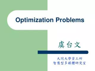
Two Discrete Optimization Problems. Problem: The Transportation Problem. Formulating Graph Problems. You already know the following steps for formulating a graph problem (such as the TSP and the Shortest-Path Problem): 1. Identify the vertices that represent objects in a problem.

E N D
Two Discrete Optimization Problems Problem: The Transportation Problem
Formulating Graph Problems You already know the following steps for formulating a graph problem (such as the TSP and the Shortest-Path Problem): 1. Identify the vertices that represent objects in a problem. 2.Identify the edges that are lines connecting selected pairs of vertices to indicated a relationship between the objects associated with the two connected vertices. 3. Identify additional data by writing those values next to the corresponding vertices and/or edges. 4. State the objective in the context of the graph and given data. Let’s do this for a new problem…
The Transportation Problem (TP) CCC has 1000 computers at each of three plants this month. Three customers have requested 1100, 800, and 1100 computers, respectively. These data are summarized in the table below, along with the cost of shipping one computer from each plant to each customer. You have been asked to develop a least-cost shipping plan for CCC.
1 1 2 2 3 3 Creating a Graph for the TP Step 1: Identify the Vertices. Use one vertex for each plant and one for each customer: Note: An edge is a relationship and not a number. Customers Plants Step 2: Identify the Edges. Use an edge to connect a vertex i to a vertex j to represent the possibility of shipping computers from Plant i to Customer j.
(Supplies) (Demands) 1 1 5 1000 1100 3 2 2 2 4 7 800 1000 8 3 6 3 7 1000 1100 4 Creating a Graph for the TP Step 3: Identify Additional Data. Plants Customers (Unit Shipping Costs)
Step 4: State the Objective You can use words, for example, for the TSP: Find the order in which to visit every vertex exactly once and return to the starting vertex with least total “cost”. OR use variables, objective function, and constraints: Step 4(a): Identify the variables, which are those quantities whose values, once determined, constitute the solution to the problem. To identify the variables, ask yourself the following questions: 1. What can you choose or control? 2. What decisions do you have to make? 3. What items affect costs or profits? 4. If you had to implement the solution, what information would you need to know?
Identifying Variables for CCC A = the number of computers to ship from P1 to C1. OR X1 = the number of computers to ship from P1 to C1. X2 = the number of computers to ship from P1 to C2. Question: What does X5mean for this problem? Note: Choose notation that is easy to understand. Xij = the number of computers to ship from Plant i to Customer j (i, j = 1, 2, 3)
Identifying the Obj. Func. For CCC Step 4(b): Identify the Objective Function (a math expression in terms of the variables and data that reflect the goal). Words: Minimize total transportation cost Decompose: Total transportation cost = Key Point: You can use decomposition more than once. Decompose (again): Transportation cost from Plant 1 = 5X11 + 3X12 + 2X13 Math: Plant 1 Plant 2 Plant 3
Identifying Constraints for CCC Step 4(c): Identify Constraints (restrictions on the values of the variables so that those values are acceptable). Note: Use grouping to identify groups of constraints. Demand Constraints ( ) 3 Words: Total number of computers received by Customer 1 should be equal to the number requested. Decompose:Total number of computers received by Customer 1 = Mathematics:
Identifying Constraints for CCC Step 4(c): Identify Constraints (cont.) Supply Constraints ( ) 3 Words: Total number of computers shipped from Plant 1 should be equal to the available supply. Decompose:Total number of computers shipped from Plant 1 = Mathematics: Logical Constraints: and integer
Transportation Problem of CCC Find values for the variables Xij(i = 1, 2, 3; j = 1, 2, 3) so as to s. t. Demand Constraints Supply Constraints 3000 3000 Qn: Is this a linear program? NO…it is an integer program. Logical Constraints Balanced TP
Means that some customers will not receive all of their demand. (Supplies) Plants Customers (Demands) 1 1 5 1000 1100 3 2 4 2 2 7 800 1000 8 6 3 3 7 1600 1000 4 0 0 0 500 3000 3500 3500 Handling Too Much Demand The algorithm for solving the transportation problem requires that total supply = total demand. Question: What do you do if total supply < total demand? Note: Shipping one unit from the Dummy Plant to Customer j means that Customer j will not receive one unit of their demand. Dum
(Supplies) Plants Customers (Demands) 1 1 5 1000 1100 3 Means that some plants will not ship all of their supplies. 2 4 2 2 7 800 1000 8 6 3 3 7 1100 1500 4 0 0 500 0 3500 3000 3500 Handling Too Much Supply The algorithm for solving the transportation problem requires that total supply = total demand. Question: What do you do if total supply > total demand? Note: Shipping one unit from Plant i to the Dummy Customer means that Plant i will have one unit of supply not shipped. Dum
x2 150 x’ = x + t*d 100 t* 50 d x1 x 50 100 Review of Simplex Alg. for LP Step 0. Initialization: Find an initial extreme point, x. This is a Finite Improvement Algorithm (FIA). Step 1. Test for Optimality: Perform a relatively easy computation to see if the current extreme point x is optimal. If so, stop. Step 2. Move: Use the fact that the current extreme point x is not optimal to: (a) DOM: Find a direction of movementd pointing from x along an edge of the feasible region that leads to improve- ment of the objective function. (b) AOM: Determine the amount t* to move from x in the direction d to reach the next extreme point. (c) Move: Move from x to x’ = x + t*d. Set x = x’ and return to Step 1.
0 0 900 800 0 100 100 0 0 0 Finding an Initial Shipping Plan Step 0 (Initialization).Find an initial shipping plan. 1000 1000 100 100 800 12600 = cost Note: Cells in which nothing is being shipped (cells 11, 12, 22, and 23) are called nonbasic cells. The others are called basic cells (cells 13, 21, 31, 32, and 33). Likewise for the variables.
The Test for Optimality +1 = cost TFO: First compute a reduced cost there for each nonbasic (“empty”) cell. The reduced costs indicates the change in the current total costs if one unit is shipped in that nonbasic cell. If the reduced cost of every nonbasic cell is ≥ 0, then the current shipping plan is optimal.
= cost Computing Reduced Costs +1 1 1 +1 +5 2 + 4 6 = +1 ≥ 0 Note: To compute rc(xij), start in cell ij and, using only the basic cells, alternate between rows and columns to find the unique “cycle” that returns to cell ij. Then, alternately add and subtract the unit shipping costs around this cycle.
= cost Not optimal Test for Optimality +1 1 +1 +1 1 1 +1 1 +1 2 + 4 7 = 2 < 0 +3 +7 4 + 6 7 = +2 > 0 +8 4 + 6 4 = +6 > 0
= cost Find the Direction of Movement Find the cycle that starts and ends at the nonbasic cell whose reduced cost is most negative (the rule of steepest descent). +1 1 1 +1
= cost Find the Amount of Movement Question: Because rc(x12) = –2, you can improve the current plan by shipping 1 unit in cell 12. In fact, each unit shipped in cell 12 reduces the costs by 2. So why not ship 1000 units there? Answer: Because each unit shipped in cell 12 requires reducing the shipment in some of the basic cells by the same amount...and the values of these basic variables cannot be reduced below 0, so t* = 800
200 +1 1 0 900 1 +1 11000 = cost Move to the New Shipping Plan Having determined that t* = 800 is the amount to ship in the chosen nonbasic cell, create the new shipping plan by adjusting the amounts shipped in each basic cell in the associated cycle. +800 800 800 +800 Note: The nonbasic cell whose value increased to t* becomes basic (cell 12, in this example) and the basic cell in the cycle whose valuedecreases to 0 becomes nonbasic (cell 32, in this example).
= cost optimal Computing Reduced Costs Again 1 +1 1 +1 1 +1 +7 4 + 6 4 + 2 3 = +4 > 0
The Stepping Stone Algorithm Step 0: (Initialization)Find an initial shipping plan x (for example, by using the Matrix Minimum Method). Step 1: (Move)Compute a reduced cost for each nonbasic cell. If all reduced costs are 0, then stop. Otherwise, choose any nonbasic cell ij whose reduced cost is < 0, create a new shipping plan as follows, and then return to Step 1: (a) Find the cycle of cells that starts and ends at cell ij. (b) Set t* = min{xij : xij is being reduced in the cycle}. (c) Starting in cell ij, alternately increase and decrease the values of the cells in the cycle by t*. The cell whose value reduces to 0 becomes nonbasic. Question: Is the final shipping plan x* obtained by the algorithm the best, that is, is x* optimal? Yes!
Variations of the Trans. Prob. • Capacitated/Uncapacitated Problems • Prohibited Routes • Transshipment Nodes • Incorporating Unequal Production Costs • Incorporating Unequal Revenue • Lower Bounds on Supplies and Demands
Summary Formulating a graph problem involves the following steps: 1. Identify the vertices by using circles to represent objects in a problem. 2.Identify the edges by using lines to connect selected pairs of vertices to indicated a relationship between the objects associated with the two connected vertices. 3. Identify other data by writing those values next to the corresponding vertices and/or edges. 4. State the objective in the context of the graph using either: • Words, or • Variables, an objective function, and constraints.
Summary The transportation problem is a combinatorial optimization problem. For a balanced problem, in which the total supply equals the total demand, the Stepping Stone Algorithm is a finite improvement algorithm that generates a sequence of shipping plans, each of which has less total cost that the preceding one. The Matrix Minimum Method is one algorithm for finding an initial feasible solution, that is, an initial shipping plan (see the next slide for details).
The Matrix Minimum Method Repeat the following steps until there are no more cells: Step 1. Identify a remaining cell ij whose unit shipping cost is the least. Step 2. Set xij = min{remaining supply at Plant i, remaining demand for Customer j}. Step 3. Reduce the supply at Plant i and the demand for Customer j by xij. Step 4. If the supply at Plant i has decreased to 0, then cross off row i. Otherwise, the demand for Customer j is now 0, so cross off column j.