Download
1 / 54
750 likes | 1.41k Views
Chapter 5: Recursion. Objectives. Looking ahead – in this chapter, we’ll consider Recursive Definitions Function Calls and Recursive Implementation Anatomy of a Recursive Call Tail Recursion Nontail Recursion Indirect Recursion Nested Recursion Excessive Recursion Backtracking.

E N D
Objectives Looking ahead – in this chapter, we’ll consider • Recursive Definitions • Function Calls and Recursive Implementation • Anatomy of a Recursive Call • Tail Recursion • Nontail Recursion • Indirect Recursion • Nested Recursion • Excessive Recursion • Backtracking Data Structures and Algorithms in C++, Fourth Edition
Recursive Definitions It is a basic rule in defining new ideas that they not be defined circularly However, it turns out that many programming constructs are defined in terms of themselves Fortunately, the formal basis for these definitions is such that no violations of the rules occurs These definitions are called recursive definitions and are often used to define infinite sets This is because an exhaustive enumeration of such a set is impossible, so some others means to define it is needed Data Structures and Algorithms in C++, Fourth Edition
Recursive Definitions (continued) • There are two parts to a recursive definition • The anchor or ground case (also sometimes called the base case) which establishes the basis for all the other elements of the set • The inductive clause which establishes rules for the creation of new elements in the set • Using this, we can define the set of natural numbers as follows: • 0 εN (anchor) • if nεN, then (n + 1) εN(inductive clause) • there are no other objects in the set N • There may be other definitions; an alternative to the previous definition is shown on page 170 Data Structures and Algorithms in C++, Fourth Edition
Recursive Definitions (continued) • We can use recursive definitions in two ways: • To define new elements in the set in question • To demonstrate that a particular item belongs in a set • Generally, the second use is demonstrated by repeated application of the inductive clause until the problem is reduced to the base case • This is often the case when we want to define functions and sequences of numbers • However this can have undesirable consequences • For example, to determine 3! (3 factorial) using a recursive definition, we have to work back to 0! Data Structures and Algorithms in C++, Fourth Edition
Recursive Definitions (continued) This results from the recursive definition of the factorial function: So 3! = 3 ∙ 2! = 3 ∙ 2 ∙ 1! = 3 ∙ 2 ∙ 1 ∙ 0! = 3 ∙ 2 ∙ 1 ∙ 1 = 6 This is cumbersome and computationally inefficient It would be helpful to find a formula that is equivalent to the recursive one without referring to previous values For factorials, we can use In general, however, this is frequently non-trivial and often quite difficult to achieve Data Structures and Algorithms in C++, Fourth Edition
Recursive Definitions (continued) These discussions and examples have been on a theoretical basis From the standpoint of computer science, recursion occurs frequently in language definitions as well as programming Fortunately, the translation from specification to code is fairly straightforward; consider a factorial function in C++: unsigned int factorial (unsigned int n){ if (n == 0) return 1; else return n * factorial (n – 1); } Data Structures and Algorithms in C++, Fourth Edition
Recursive Definitions (continued) Although the code is simple, the underlying ideas supporting its operation are quite involved Fortunately, most modern programming languages incorporate mechanisms to support the use of recursion, making it transparent to the user Typically, recursion is supported through use of the runtime stack So to get a clearer understanding of recursion, we will look at how function calls are processed Data Structures and Algorithms in C++, Fourth Edition
Function Calls and Recursive Implementation What kind of information must we keep track of when a function is called? If the function has parameters, they need to be initialized to their corresponding arguments In addition, we need to know where to resume the calling function once the called function is complete Since functions can be called from other functions, we also need to keep track of local variables for scope purposes Because we may not know in advance how many calls will occur, a stack is a more efficient location to save information Data Structures and Algorithms in C++, Fourth Edition
Function Calls and Recursive Implementation (continued) • So we can characterize the state of a function by a set of information, called an activation record or stack frame • This is stored on the runtime stack, and contains the following information: • Values of the function’s parameters, addresses of reference variables (including arrays) • Copies of local variables • The return address of the calling function • A dynamic link to the calling function’s activation record • The function’s return value if it is not void • Every time a function is called, its activation record is created and placed on the runtime stack Data Structures and Algorithms in C++, Fourth Edition
Function Calls and Recursive Implementation (continued) So the runtime stack always contains the current state of the function As an illustration, consider a function f1()called from main() It in turn calls function f2(), which calls function f3() The current state of the stack, with function f3()executing, is shown in Figure 5.1 Once f3()completes, its record is popped, and function f2()can resume and access information in its record If f3()calls another function, the new function has its activation record pushed onto the stack as f3()is suspended Data Structures and Algorithms in C++, Fourth Edition
Function Calls and Recursive Implementation (continued) Fig. 5.1 Contents of the run-time stack when main() calls function f1(), f1() calls f2(), and f2() calls f3() Data Structures and Algorithms in C++, Fourth Edition
Function Calls and Recursive Implementation (continued) The use of activation records on the runtime stack allows recursion to be implemented and handled correctly Essentially, when a function calls itself recursively, it pushes a new activation record of itself on the stack This suspends the calling instance of the function, and allows the new activation to carry on the process Thus, a recursive call creates a series of activation records for different instances of the same function Data Structures and Algorithms in C++, Fourth Edition
Anatomy of a Recursive Call To gain further insight into the behavior of recursion, let’s dissect a recursive function and analyze its behavior The function we will look at is defined in the text, and can be used to raise a number x to a non-negative integer power n: We can also represent this function using C++ code, shown on the next slide Data Structures and Algorithms in C++, Fourth Edition
Anatomy of a Recursive Call (continued) /* 102 */ double power (double x, unsigned int n) { /* 103 */ if (n == 0) /* 104 */ return 1.0; else /* 105 */ return x * power(x,n-1); } Using the definition, the calculation of x4 would be calculated as follows: x4 = x ∙ x3 = x ∙ (x ∙ x2) =x ∙ (x ∙ (x ∙ x1)) = x ∙ (x ∙ (x ∙ (x ∙ x0))) = x ∙ (x ∙ (x ∙ (x ∙ 1))) = x ∙ (x ∙ (x ∙ (x))) = x ∙ (x ∙ (x ∙ x)) = x ∙ (x ∙ x∙ x) = x ∙ x∙ x∙ x Notice how repeated application of the inductive step leads to the anchor Data Structures and Algorithms in C++, Fourth Edition
Anatomy of a Recursive Call (continued) This produces the result of x0, which is 1, and returns this value to the previous call That call, which had been suspended, then resumes to calculate x ∙ 1, producing x Each succeeding return then takes the previous result and uses it in turn to produce the final result The sequence of recursive calls and returns looks like: call 1x4 = x ∙ x3 = x ∙ x ∙ x ∙ x call 2x3 = x ∙ x2 = x ∙ x ∙ x call 3x2 = x ∙ x1 = x ∙ x call 4x1 = x ∙ x0 = x ∙ 1 call 5x0 = 1 Data Structures and Algorithms in C++, Fourth Edition
Anatomy of a Recursive Call (continued) Now, the sequence of calls is kept track of on the runtime stack, which stores the return address of the function call This is used to remember where to resume execution after the function has completed The function power()in the earlier slide is called by the following statement: /* 136 */ y = power(5.6,2); The sequence of calls and returns generated by this call, along with the address of the calling statement, the return address, and the arguments, are shown in Figure 5.2 Data Structures and Algorithms in C++, Fourth Edition
Anatomy of a Recursive Call (continued) Fig. 5.2 Changes to the run-time stack during execution of power(5.6,2) Data Structures and Algorithms in C++, Fourth Edition
Anatomy of a Recursive Call (continued) The initial call (Figure 5.2a) shows the arguments (5.6 and 2), the return address (136), and the space for the return value The exponent is greater than 0, so the else clause is executed; the function calls itself with arguments (5.6 and 1) This causes a new activation record to be added to the stack, as shown in Figure 5.2b Since the exponent is 1, the elseclause again calls the function with arguments (5.6 and 0), adding another activation record to the stack (figure 5.2c) This time, the value of the exponent is 0, so the function returns the value 1 (Figures 5.2d and 5.2e) Data Structures and Algorithms in C++, Fourth Edition
Anatomy of a Recursive Call (continued) This causes the current activation record to be popped from the stack (notice the location of the stack pointer) The previous call to the function now resumes, and calculates 5.6 * the result of the call, which is 1, resulting in 5.6 This is placed in the activation record, and the call completes, popping the stack again (Figures 5.2f and 5.2g) Finally, the original call to the function completes by multiplying 5.6 * the call result (5.6), resulting in 31.36 This is placed in the activation record, and when this call completes, the value is returned to the original call in line 136 (Figure 5.2h) Data Structures and Algorithms in C++, Fourth Edition
Anatomy of a Recursive Call (continued) It is possible to implement the power() function in a non-recursive manner, as shown below: double nonRecPower(double x, unsigned int n) { double result = 1; for (result = x; n > 1; --n) result *= x; return result; } However, in comparing this to the recursive version, we can see that the recursive code is more intuitive, closer to the specification, and simpler to code Data Structures and Algorithms in C++, Fourth Edition
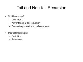
Tail Recursion The nature of a recursive definition is that the function contains a reference to itself This reference can take on a number of different forms We’re going to consider a few of these, starting with the simplest, tail recursion The characteristic implementation of tail recursion is that a single recursive call occurs at the end of the function No other statements follow the recursive call, and there are no other recursive calls prior to the call at the end of the function Data Structures and Algorithms in C++, Fourth Edition
Tail Recursion (continued) An example of a tail recursive function is the code: void tail(int i) { if (i > 0) { cout << i << ''; tail(i-1); } } Essentially, tail recursion is a loop; it can be replaced by an iterative algorithm to accomplish the same task In fact, in most cases, languages supporting loops should use this construct rather than recursion Data Structures and Algorithms in C++, Fourth Edition
Tail Recursion (continued) An example of an iterative form of the function is shown below: void iterativeEquivalentOfTail(int i) { for ( ; i > 0; i--) cout << i << ''; } Data Structures and Algorithms in C++, Fourth Edition
Nontail Recursion As an example of another type of recursion, consider the following code from page 178 of the text: /* 200 */ void reverse() { char ch; /* 201 */ cin.get(ch); /* 202 */ if (ch != '\n') { /* 203 */ reverse(); /* 204 */ cout.put(ch); } } The function displays a line of input in reverse order Data Structures and Algorithms in C++, Fourth Edition
Nontail Recursion (continued) To accomplish this, the function reverse() uses recursion to repeatedly call itself for each character in the input line Assuming the input “ABC”, the first time reverse() is called an activation record is created to store the local variable ch and the return address of the call in main() This is shown in Figure 5.3a The get() function (line 201) reads in the character “A” from the line and compares it with the end-of-line character Since they aren’t equal, the function calls itself in line 203, creating a new activation record shown in Figure 5.3b Data Structures and Algorithms in C++, Fourth Edition
Nontail Recursion (continued) Fig. 5.3 Changes on the run-time stack during the execution of reverse() This process continues until the end of line character is read and the stack appears as in Figure 5.3d At this point, the current call terminates, popping the last activation record off the stack, and resuming the previous call at line 204 Data Structures and Algorithms in C++, Fourth Edition
Nontail Recursion (continued) This line outputs the current value of ch, which is contained in the current activation record, and is the value “C” The current call then ends, causing a repeat of the pop and return action, and once again the output is executed displaying the character “B” Finally, the original call to reverse() is reached, which will output the character “A” At that point, control is returned to main(), and the string “CBA” will be displayed This type of recursion, where the recursive call precedes other code in the function, is called nontail recursion Data Structures and Algorithms in C++, Fourth Edition
Nontail Recursion (continued) Now consider a non-recursive version of the same algorithm: void simpleIterativeReverse() { char stack[80]; register int top = 0; cin.getline(stack,80); for(top = strlen(stack)-1; top >= 0; cout.put(stack[top--])); } This version utilizes functions from the standard C++ library to handle the input and string reversal So the details of the process are hidden by the functions Data Structures and Algorithms in C++, Fourth Edition
Nontail Recursion (continued) If these functions weren’t available, we’d have to make the processing more explicit, as in the following code: void iterativeReverse() { char stack[80]; register int top = 0; cin.get(stack[top]); while(stack[top]!='\n') cin.get(stack[++top]); for (top -= 2; top >= 0; cout.put(stack[top--])); } Data Structures and Algorithms in C++, Fourth Edition
Nontail Recursion (continued) In this code, we can see explicitly how the input is handled, using an array to simulate the run-time stack behavior The first get() retrieves the first character from input, and the loop implements the getline()function operation When the end-of-line character is detected, the loop terminates, and the array contains the characters entered The for loop then adjusts the top value to the last character before the end-of-line, and runs backward through the array, outputting the characters in reverse order Data Structures and Algorithms in C++, Fourth Edition
Nontail Recursion (continued) These iterative versions illustrate several important points First, when implementing nontail recursion iteratively, the stack must be explicitly implemented and handled Second, the clarity of the algorithm, and often its brevity, are sacrificed as a consequence of the conversion Therefore, unless compelling reasons are evident during the algorithm design, we typically use the recursive versions Data Structures and Algorithms in C++, Fourth Edition
Indirect Recursion The previous discussions have focused on situations where a function, f(), invokes itself recursively (direct recursion) However, in some situations, the function may be called not by itself, but by a function that it calls, forming a chain: f()→ g() → f() This is known as indirect recursion The chains of calls may be of arbitrary length, such as: f()→ f1()→ f2() → ∙∙∙ → fn()→ f() It is also possible that a given function may be a part of multiple chains, based on different calls Data Structures and Algorithms in C++, Fourth Edition
Indirect Recursion (continued) So our previous chain might look like: f1() → f2() → ∙∙∙ → fn() ↗ ↘ f() f() ↘ ↗ g1() → g2() → ∙∙∙ → gm() Data Structures and Algorithms in C++, Fourth Edition
Nested Recursion Another interesting type of recursion occurs when a function calls itself and is also one of the parameters of the call Consider the example shown on page 186 of the text: From this definition, it is given that the function has solutions for n = 0 and n > 4 However, for n = 1, 2, 3, and 4, the function determines a value based on a recursive call that requires evaluating itself This is called nested recursion Data Structures and Algorithms in C++, Fourth Edition
Nested Recursion (continued) Another example is the famous (or perhaps infamous) Ackermann function, defined as: First suggested by Wilhelm Ackermann in 1928 and later modified by Rosza Peter, it is characterized by its rapid growth To get a sense of this growth, consider that A(3,m) = 2m+3 – 3, and Data Structures and Algorithms in C++, Fourth Edition
Nested Recursion (continued) There are (m – 1) 2s in the exponent, so A(4,1) = 216 - 3, which is 65533 However, changing m to 2 has a dramatic impact as the value of has 19,729 digits in its expansion As can be inferred from this, the function is elegantly expressed recursively, but quite a problem to define iteratively Data Structures and Algorithms in C++, Fourth Edition
Excessive Recursion Recursive algorithms tend to exhibit simplicity in their implementation and are typically easy to read and follow However, this straightforwardness does have some drawbacks Generally, as the number of function calls increases, a program suffers from some performance decrease Also, the amount of stack space required increases dramatically with the amount of recursion that occurs This can lead to program crashes if the stack runs out of memory More frequently, though, is the increased execution time leading to poor program performance Data Structures and Algorithms in C++, Fourth Edition
Excessive Recursion (continued) As an example of this, consider the Fibonacci numbers They are first mentioned in connection with Sanskrit poetry as far back as 200 BCE Leonardo Pisano Bigollo (also known as Fibonacci), introduced them to the western world in his book Liber Abaci in 1202 CE The first few terms of the sequence are 0, 1, 1, 2, 3, 5, 8, … and can be generated using the function: Data Structures and Algorithms in C++, Fourth Edition
Excessive Recursion (continued) This tells us that that any Fibonacci number after the first two (0 and 1) is defined as the sum of the two previous numbers However, as we move further on in the sequence, the amount of calculation necessary to generate successive terms becomes excessive This is because every calculation ultimately has to rely on the base case for computing the values, since no intermediate values are remembered The following algorithm implements this definition; again, notice the simplicity of the code that belies the underlying inefficiency Data Structures and Algorithms in C++, Fourth Edition
Excessive Recursion (continued) unsigned long Fib(unsigned long n) { if (n < 2) return n; // else return Fib(n-2) + Fib(n-1); } If we use this to compute Fib(6)(which is 8), the algorithm starts by calculating Fib(4) + Fib(5) The algorithm then needs to calculate Fib(4) = Fib(2) + Fib(3), and finally the first term of that is Fib(2) = Fib(0) + Fib(1)= 0 + 1 = 1 Data Structures and Algorithms in C++, Fourth Edition
Excessive Recursion (continued) The entire process can be represented using a tree to show the calculations: Fig. 5.8 The tree of calls for Fib(6). Counting the branches, it takes 25 calls to Fib() to calculate Fib(6) Data Structures and Algorithms in C++, Fourth Edition
Excessive Recursion (continued) The total number of additions required to calculate the nthnumber can be shown to be Fib(n + 1) – 1 With two calls per addition, and the first call taken into account, the total number of calls is 2 ∙ Fib(n + 1) – 1 Values of this are shown in the following table: Fig. 5.9 Number of addition operations and number of recursive calls to calculate Fibonacci numbers. Data Structures and Algorithms in C++, Fourth Edition
Excessive Recursion (continued) Notice that it takes almost 3 million calls to determine the 31st Fibonacci number This exponential growth makes the algorithm unsuitable for anything but small values of n Fortunately there are acceptable iterative algorithms that can be used far more effectively However, there is an even more useful arithmetic technique, known as Binet’s formula, although first developed by Abraham de Moivre: Data Structures and Algorithms in C++, Fourth Edition
Excessive Recursion (continued) In this formula, and Since the second term is between -1 and 0, it becomes very small as n grows, so it can be ignored in the formula, which becomes: This can be rounded to the nearest integer to produce the Fibonacci number This formula also has a very straightforward implementation in code, using the ceil() function to round the result to the nearest integer Data Structures and Algorithms in C++, Fourth Edition
Excessive Recursion (continued) unsigned long deMoivreFib(unsigned long n) { return ceil(exp(n*log(1.6180339897)- log(2.2360679775))-0.5); } Data Structures and Algorithms in C++, Fourth Edition
Backtracking Backtracking is an approach to problem solving that uses a systematic search among possible pathways to a solution As each path is examined, if it is determined the pathway isn’t viable, it is discarded and the algorithm returns to the prior branch so that a different path can be explored Thus, the algorithm must be able to return to the previous position, and ensure that all pathways are examined Backtracking is used in a number of applications, including artificial intelligence, compiling, and optimization problems One classic application of this technique is known as The Eight Queens Problem Data Structures and Algorithms in C++, Fourth Edition
Backtracking (continued) In this problem, we try to place eight queens on a chessboard in such a way that no two queens attack each other Fig. 5.11 The eight queens problem Data Structures and Algorithms in C++, Fourth Edition
Backtracking (continued) The approach to solving this is to place one queen at a time, trying to make sure that the queens do not check each other If at any point a queen cannot be successfully placed, the algorithm backtracks to the placement of the previous queen This is then moved and the next queen is tried again If no successful arrangement is found, the algorithm backtracks further, adjusting the previous queen’s predecessor, etc. A pseudocode representation of the backtracking algorithm is shown in the next slide; the process is described in detail on pages 192 – 197, along with a C++ implementation Data Structures and Algorithms in C++, Fourth Edition
Backtracking (continued) putQueen(row) for every position col on the same row if position col is available place the next queen in position col; if (row < 8) putQueen(row+1); else success; remove the queen from position col; This algorithm will find all solutions, although some are symmetrical Data Structures and Algorithms in C++, Fourth Edition