Multiple Sequence Alignment (III) and Evolution/Phylogenetic methods

1. C E N T E R F O R I N T E G R A T I V E B I O I N F O R M A T I C S V U Introduction to bioinformatics 2007Lecture 11 Multiple Sequence Alignment (III)and Evolution/Phylogenetic methods

2. Evaluating multiple alignments • There are reference databases based on structural information: e.g. BAliBASE and HOMSTRAD • Conflicting standards of truth • evolution • structure • function • With orphan sequences no additional information • Benchmarks depending on reference alignments • Quality issue of available reference alignment databases • Different ways to quantify agreement with reference alignment (sum-of-pairs, column score) • “Charlie Chaplin” problem

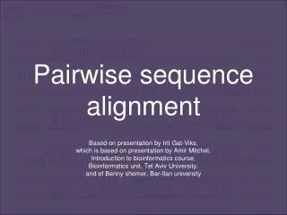
3. Evaluating multiple alignments • As a standard of truth, often a reference alignment based on structural superpositioning is taken These superpositionings can be scored using the root-mean-square-deviation (RMSD) of atoms that are equivalenced (taken as corresponding) in a pair of protein structures

4. BAliBASE benchmark alignments Thompson et al. (1999) NAR 27, 2682. • 8 categories: • cat. 1 - equidistant • cat. 2 - orphan sequence • cat. 3 - 2 distant groups • cat. 4 – long overhangs • cat. 5 - long insertions/deletions • cat. 6 – repeats • cat. 7 – transmembrane proteins • cat. 8 – circular permutations

5. . . . BAliBASE BB11001 1aab_ref1Ref1 V1 SHORT high mobility group protein BB11002 1aboA_ref1 Ref1 V1 SHORT SH3 BB11003 1ad3_ref1 Ref1 V1 LONG aldehyde dehydrogenase BB11004 1adj_ref1 Ref1 V1 LONG histidyl-trna synthetase BB11005 1ajsA_ref1 Ref1 V1 LONG aminotransferase BB11006 1bbt3_ref1 Ref1 V1 MEDIUM foot-and-mouth disease virus BB11007 1cpt_ref1 Ref1 V1 LONG cytochrome p450 BB11008 1csy_ref1 Ref1 V1 SHORT SH2 BB11009 1dox_ref1 Ref1 V1 SHORT ferredoxin [2fe-2s]

6. T-Coffee: correctly aligned Kinase nucleotide binding sites

7. Scoring a single MSA with the Sum-of-pairs (SP) score Good alignments should have a high SP score, but it is not always the case that the true biological alignment has the highest score. • Sum-of-Pairs score • Calculate the sum of all pairwise alignment scores • This is equivalent to taking the sum of all matched a.a. pairs • The latter can be done using gap penalties or not

8. Evaluation measures Query Reference Column score What fraction of the MSA columns in the reference alignment is reproduced by the computed alignment Sum-of-Pairs score What fraction of the matched amino acid pairs in the reference alignment is reproduced by the computed alignment

9. Evaluating multiple alignments

10. Evaluating multiple alignmentsCharlie Chaplin problem SP BAliBASE alignment nseq * len

11. Evaluating multiple alignmentsCharlie Chaplin problem

12. Comparing T-coffee with other methods

13. BAliBASE benchmark alignments

14. Summary • Individual alignments can be scored with the SP score. • Better alignments should have better SP scores • However, there is the Charlie Chaplin problem • A test and a reference multiple alignment can be scored using the SP score or the column score (now for pairs of alignments) • Evaluations show that there is no MSA method that always wins over others in terms of alignment quality

15. Lecture 11:Evolution/Phylogeny methods Introduction to Bioinformatics

16. Bioinformatics • “Nothing in Biology makes sense except in the light of evolution” (Theodosius Dobzhansky (1900-1975)) • “Nothing in bioinformatics makes sense except in the light of Biology”

17. Evolution • Most of bioinformatics is comparative biology • Comparative biology is based upon evolutionary relationships between compared entities • Evolutionary relationships are normally depicted in a phylogenetic tree

18. Where can phylogeny be used • For example, finding out about orthology versus paralogy • Predicting secondary structure of RNA • Studying host-parasite relationships • Mapping cell-bound receptors onto their binding ligands • Multiple sequence alignment (e.g. Clustal)

19. DNA evolution • Gene nucleotide substitutions can be synonymous (i.e. not changing the encoded amino acid) or nonsynonymous (i.e. changing the a.a.). • Rates of evolution vary tremendously among protein-codinggenes. Molecular evolutionary studies have revealed an∼1000-fold range of nonsynonymous substitution rates (Liand Graur 1991). • The strength of negative (purifying) selectionis thought to be the most important factor in determiningthe rate of evolution for the protein-coding regions of agene (Kimura 1983; Ohta 1992; Li 1997).

20. DNA evolution • “Essential” and “nonessential” are classic moleculargenetic designations relating to organismal fitness. • A gene is considered to be essential if a knock-outresults in (conditional) lethality or infertility. • Nonessential genes are those for which knock-outs yieldviable and fertile individuals. • Given the role of purifyingselection in determining evolutionary rates, thegreater levels of purifying selection on essential genes leads to a lower rate of evolution relative to that ofnonessential genes.

21. Reminder -- Orthology/paralogy Orthologous genes are homologous (corresponding) genes in different species Paralogous genes are homologous genes within the same species (genome)

22. Old Dogma – Recapitulation Theory (1866) Ernst Haeckel: “Ontogeny recapitulates phylogeny” Ontogeny is the development of the embryo of a given species; phylogeny is the evolutionary history of a species http://en.wikipedia.org/wiki/Recapitulation_theory Haeckels drawing in support of his theory: For example, the human embryo with gill slits in the neck was believed by Haeckel to not only signify a fishlike ancestor, but it represented a total fishlike stage in development. Gill slits are not the same as gills and are not functional.

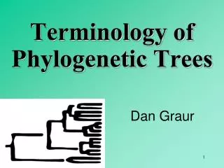
23. Phylogenetic tree (unrooted) human Drosophila internal node fugu mouse leaf OTU – Observed taxonomic unit edge

24. Phylogenetic tree (unrooted) root human Drosophila internal node fugu mouse leaf OTU – Observed taxonomic unit edge

25. Phylogenetic tree (rooted) root time edge internal node (ancestor) leaf OTU – Observed taxonomic unit Drosophila human fugu mouse

26. How to root a tree m f • Outgroup – place root between distant sequence and rest group • Midpoint – place root at midpoint of longest path (sum of branches between any two OTUs) • Gene duplication – place root between paralogous gene copies h D f m h D 1 m f 3 1 2 4 2 3 1 1 1 h 5 D f m h D f- f- h- f- h- f- h- h-

27. Combinatoric explosion Number of unrooted trees = Number of rooted trees =

28. Combinatoric explosion # sequences # unrooted # rooted trees trees 2 1 1 3 1 3 4 3 15 5 15 105 6 105 945 7 945 10,395 8 10,395 135,135 9 135,135 2,027,025 10 2,027,025 34,459,425

29. Tree distances Evolutionary (sequence distance) = sequence dissimilarity 5 human x mouse 6 x fugu 7 3 x Drosophila 14 10 9 x human 1 mouse 2 1 1 fugu 6 Drosophila mouse Drosophila human fugu Note that with evolutionary methods for generating trees you get distances between objects by walking from one to the other.

30. Phylogeny methods • Distance based – pairwise distances (input is distance matrix) • Parsimony – fewest number of evolutionary events (mutations) – relatively often fails to reconstruct correct phylogeny, but methods have improved recently • Maximum likelihood – L = Pr[Data|Tree] – most flexible class of methods - user-specified evolutionary methods can be used

31. Distance based --UPGMA Let Ci andCj be two disjoint clusters: 1 di,j = ————————pqdp,q, where p  Ci and q  Cj |Ci| × |Cj| Ci Cj In words: calculate the average over all pairwise inter-cluster distances

32. Clustering algorithm: UPGMA • Initialisation: • Fill distance matrix with pairwise distances • Start with N clusters of 1 element each • Iteration: • Merge cluster Ci and Cj for which dij is minimal • Place internal node connecting Ci and Cj at height dij/2 • Delete Ci and Cj (keep internal node) • Termination: • When two clusters i, j remain, place root of tree at height dij/2 d

33. Ultrametric Distances • A tree T in a metric space (M,d) where d is ultrametric has the following property: there is a way to place a root on T so that for all nodes in M, their distance to the root is the same. Such T is referred to as a uniformmolecular clock tree. • (M,d) is ultrametric if for every set of three elements i,j,k∈M, two of the distances coincide and are greater than or equal to the third one (see next slide). • UPGMA is guaranteed to build correct tree if distances are ultrametric. But it fails if not!

34. Ultrametric Distances Given three leaves, two distances are equal while a third is smaller: d(i,j)  d(i,k) = d(j,k) a+a  a+b = a+b i nodes i and j are at same evolutionary distance from k – dendrogram will therefore have ‘aligned’ leafs; i.e. they are all at same distance from root a b k a j

35. Evolutionary clock speeds Uniform clock: Ultrametric distances lead to identical distances from root to leafs Non-uniform evolutionary clock: leaves have different distances to the root -- an important property is that of additive trees. These are trees where the distance between any pair of leaves is the sum of the lengths of edges connecting them. Such trees obey the so-called 4-point condition (next slide).

36. Additive trees All distances satisfy 4-point condition: For all leaves i,j,k,l: d(i,j)+ d(k,l)  d(i,k) + d(j,l) = d(i,l) + d(j,k) (a+b)+(c+d)  (a+m+c)+(b+m+d) = (a+m+d)+(b+m+c) k i a c m b d j l Result: all pairwise distances obtained by traversing the tree

37. Additive trees • In additive trees, the distance between any pair of leaves is the sum of lengths of edges connecting them • Given a set of additive distances: a unique tree T can be constructed: • For two neighbouring leaves i,j with common parent k, place parent node k at a distance from any node m with • d(k,m) = ½ (d(i,m) + d(j,m) – d(i,j)) • c = ½ ((a+c) + (b+c) – (a+b)) i a c m k b j d is ultrametric ==> d additive

38. Distance based --Neighbour-Joining (Saitou and Nei, 1987) • Guaranteed to produce correct tree if distances are additive • May even produce good tree if distances are not additive • Global measure – keeps total branch length minimal • At each step, join two nodes such that the total tree length (sum of all branch lengths) is minimal (criterion of minimal evolution) • Agglomerative algorithm • Leads to unrooted tree

39. Neighbour joining y x x x y (c) (a) (b) x x x y y (f) (d) (e) At each step all possible ‘neighbour joinings’ are checked and the one corresponding to the minimal total tree length (calculated by adding all branch lengths) is taken.

40. Algorithm: Neighbour joining • NJ algorithm in words: • Make star tree with ‘fake’ distances (we need these to be able to calculate total branch length) • Check all n(n-1)/2 possible pairs and join the pair that leads to smallest total branch length. You do this for each pair by calculating the real branch lengths from the pair to the common ancestor node (which is created here – ‘y’ in the preceding slide) and from the latter node to the tree • Select the pair that leads to the smallest total branch length (by adding up real and ‘fake’ distances). Record and then delete the pair and their two branches to the ancestral node, but keep the new ancestral node. The tree is now 1 one node smaller than before. • Go to 2, unless you are done and have a complete tree with all real branch lengths (recorded in preceding step)

41. Neighbour joining Finding neighbouring leaves: Define Dij = dij – (ri + rj) Where 1 ri = ——— k dik |L| - 2 Total tree length Dij is minimal iff i and j are neighbours Proof in Durbin book, p. 189

42. Algorithm: Neighbour joining • Initialisation: • Define T to be set of leaf nodes, one per sequence • Let L = T • Iteration: • Pick i,j (neighbours) such that Di,j is minimal (minimal total tree length) • Define new node k, and set dkm = ½ (dim + djm – dij) for all m  L • Add k to T, with edges of length dik = ½ (dij + ri – rj) • Remove i,j from L; Add k to L • Termination: • When L consists of two nodes i,j and the edge between them of length dij

43. Parsimony & Distance parsimony Sequences 1 2 3 4 5 6 7 Drosophila t t a t t a a fugu a a t t t a a mouse a a a a a t a human a a a a a a t Drosophila mouse 1 6 4 5 2 3 7 human fugu distance human x mouse 2 x fugu 4 4 x Drosophila5 5 3 x Drosophila 2 mouse 1 2 1 1 human fugu mouse Drosophila human fugu

44. Problem: Long Branch Attraction (LBA) • Particular problem associated with parsimony methods • Rapidly evolving taxa are placed together in a tree regardless of their true position • Partly due to assumption in parsimony that all lineages evolve at the same rate • This means that also UPGMA suffers from LBA • Some evidence exists that also implicates NJ A A B D C B D Inferred tree C True tree

45. Maximum likelihoodPioneered by Joe Felsenstein • If data=alignment, hypothesis = tree, and under a given evolutionary model, maximum likelihood selects the hypothesis (tree) that maximises the observed data • A statistical (Bayesian) way of looking at this is that the tree with the largest posterior probability is calculated based on the prior probabilities; i.e. the evolutionary model (or observations). • Extremely time consuming method • We also can test the relative fit to the tree of different models (Huelsenbeck & Rannala, 1997)

46. Maximum likelihood Methods to calculate ML tree: • Phylip (http://evolution.genetics.washington.edu/phylip.html) • Paup (http://paup.csit.fsu.edu/index.html) • MrBayes (http://mrbayes.csit.fsu.edu/index.php) Method to analyse phylogenetic tree with ML: • PAML (http://abacus.gene.ucl.ac.uk/software/paml.htm) The strength of PAML is its collection of sophisticated substitution models to analyse trees. • Programs such as PAML can test the relative fit to the tree of different models (Huelsenbeck & Rannala, 1997)

47. Maximum likelihood • A number of ML tree packages (e.g. Phylip, PAML) contain tree algorithms that include the assumption of a uniform molecular clock as well as algorithms that don’t • These can both be run on a given tree, after which the results can be used to estimate the probability of a uniform clock.

48. How to assess confidence in tree

49. How to assess confidence in tree • Distance method – bootstrap: • Select multiple alignment columns with replacement (scramble the MSA) • Recalculate tree • Compare branches with original (target) tree • Repeat 100-1000 times, so calculate 100-1000 different trees • How often is branching (point between 3 nodes) preserved for each internal node in these 100-1000 trees? • Bootstrapping uses resampling of the data

50. The Bootstrap -- example Used multiple times in resampled (scrambled) MSA below 1 2 3 4 5 6 7 8 - C V K V I Y S M A V R - I F S M C L R L L F T 3 4 3 8 6 6 8 6 V K V S I I S I V R V S I I S I L R L T L L T L 5 1 2 3 Original 4 2x 3x 1 1 2 3 Non-supportive Scrambled 5 Only boxed alignment columns are randomly selected in this example