Download
1 / 49
490 likes | 604 Views
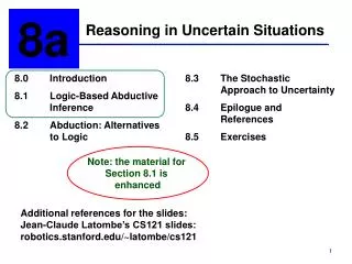
Ch9 Reasoning in Uncertain Situations. Dr. Bernard Chen Ph.D. University of Central Arkansas Spring 2011. Outline . Reasoning in Fuzzy Sets Markov Models. Reasoning with Fuzzy Sets. There are two assumptions that are essential for the use of formal set theory:

E N D
Ch9 Reasoning in Uncertain Situations Dr. Bernard Chen Ph.D. University of Central Arkansas Spring 2011
Outline • Reasoning in Fuzzy Sets • Markov Models
Reasoning with Fuzzy Sets • There are two assumptions that are essential for the use of formal set theory: • For any element and a set belonging to some universe, the element is either a member of the set or else it is a member of the complement of that set • An element cannot belong to both a set and also to its complement
Reasoning with Fuzzy Sets • Both these assumptions are violated in Lotif Zadeh.s fuzzy set theory • Zadeh.s main contention (1983) is that, although probability theory is appropriate for measuring randomness of information, it is inappropriate for measuring the meaning of the information • Zadeh proposes possibility theoryas a measure of vagueness, just like probability theory measures randomness
Reasoning with Fuzzy Sets • The notation of fuzzy set can be describes as follows: let S be a set and s a member of that set, A fuzzy subset F od S is defined by a membership function mF(s) that measures the “degree” to which s belongs to F
Reasoning with Fuzzy Sets • For example: • S to be the set of positive integers and F to be the fuzzy subset of S called small integers • Now, various integer values can have a “possibility” distribution defining their “fuzzy membership” in the set of small integers: mF(1)=1.0, mF(3)=0.9, mF(50)=0.001
Reasoning with Fuzzy Sets • For the fuzzy set representation of the set of small integers, in previous figure, each integer belongs to this set with an associated confidence measure. • In the traditional logic of “crisp” set, the confidence of an element being in a set must be either 1 or 0
Reasoning with Fuzzy Sets • This figure offers a set membership function for the concept of short, medium, and tall male humans. • Note that any one person can belong to more than one set • For example, a 5.9” male belongs to both the set of medium as well as to the set of tall males
Reasoning with Fuzzy Sets • A classic in the fuzzy set literature, a control regime for an inverted pendulum • We desire to keep in balance and pointing upward • We keep the pendulum in balance by moving the base of the system to offset the force of gravity acting on the pendulum
Reasoning with Fuzzy Sets • We simplify the problem by presenting it in 2D • There are two measurements are used as input values to the controller • First angle θ, the deviation of the pendulum from the vertical • Second, the speed dθ/dt, at which the pendulum is moving • Both measures are positive in the quadrant to the right and negative to the left
Reasoning with Fuzzy Sets • The input value θ is partitioned into three regions: Negative, Zero, and Positive • The input value dθ/dt is also partitioned into three regions: Negative, Zero, and Positive
Reasoning with Fuzzy Sets • This figure is the defuzzified control response, where we use middle five regions, Negative Big, Negitive, Positive, Positive Big • Note that both the original input and final output data of the controller are crisp value
Reasoning with Fuzzy Sets • How to use this??? • For example, if we currently we have the situation: θ=1 ; dθ/dt=-4
Reasoning with Fuzzy Sets • For θ, the value are Zero with 0.5 and Positive with 0.5 • For dθ/dt, the value are Negative with 0.8 and Zero with 0.2 • The Fuzzy Associative Matrix (FAM) for the pendulum problem. The input values are on the left and top
Reasoning with Fuzzy Sets • In this case, because each input value touched on two regions of the input space, four rules must be applied • Dr. Zedah is the first to propose these combination rules for the algebra of fuzzy reasoning • In our example, all premise pairs are ANDed together, so the minimum of their measures is taken as the measure of the rule result
Outline • Reasoning in Fuzzy Sets • Markov Models
So how is “Tomato” pronounced • A probabilistic finite state acceptor for the pronunciation of “tomato”, adapted from Jurafsky and Martin (2000).
Markov Models • In section 5.3, we presented the probabilistic finite state machine • A state machine where the next state function was represented by probability distribution on the current state • The discrete Markov process is a specialization of this approach, where the system ignores its input values
Markov Models • NO body understands it… • Lets take a look of an example: • S1= Sun • S2= Cloudy • S3= Fog • S4= Precipitation
Markov Models • S1= Sun • S2= Cloudy • S3= Fog • S4= Precipitation
Markov Models • We now are able to ask questions of our model. • Suppose today, S1, is sunny, • What is the probability of the next five days remaining Sunny? • What is the probibility of the next five days being sunny, sunny, cloudy, cloudy, precipitation?
Markov Models • Answer for the first question: • 0.4^5 • Answer for the second question:
Markov Models • Use Markov Model to represent the idea
Markov Models • This example follows the “first-order” Markov assumption where weather each day is a function (only) of the weather the day before • We also observe the fact that today is sunshine !? (Fuzzy concept may be applied)
Markov Models • We may also extend this example to determine, given that we know today.s weather, the probability that the weather will be the same for exactly the next t days • O={si (today), si, …, si, sj}, where there are exactly (t+1) si, and si!=sj, then: • p(O|M)=1*aii^t*(1-aii)
Markov Models • There are many advanced Markov Models • Hidden Markov Models • Semi-Markov Models • Markov Decision Processes
Markov Chains Rain Cloudy Sunny State transition matrix States Initial Distribution Sunny Cloud Rain 1 0 0
Hidden Markov Models Hidden states : the (TRUE) states of a system that may be described by a Markov process (e.g., the weather). Observable states : the states of the process that are `visible. (e.g., seaweed dampness).
Components Of HMM Initial Distribution : contains the probability of the (hidden) model being in a particular hidden state at time t = 1. State transition matrix : holding the probability of a hidden state given the previous hidden state.
Hidden Markov Models • Question now we may ask is like: Today is a Dryish day, what is tomorrow.s weather might be?
Hidden Markov Models • Since today is a Dryish day, we know that: • Sun 20/ • Cloud 30/ • Rain 20/
Hidden Markov Models • Therefore: The opportunity of Sunny: 0.01+0.12+0.04=0.17 Cloudy: 0.06+0.06+0.10=0.22 Rain: 0.04+0.12+0.06=0.22 Tomorrow is Rain or Cloudy
Amherst Application of HMM • HMMs are very common in Computational Linguistics: • Speech recognition (observed: acoustic signal, hidden: words) • Handwriting recognition (observed: image, hidden: words) • Part-of-speech tagging (observed: words, hidden: part-of-speech tags) • Machine translation (observed: foreign words, hidden: words in target language)
Application of HMM • Biology • Gene finding and prediction • Protein-Profile Analysis • Secondary Structure prediction
Building – from an existing alignment ACA - - - ATG TCA ACT ATC ACA C - - AGC AGA - - - ATC ACC G - - ATC insertion Transition probabilities Output Probabilities A HMM model for a DNA motif alignments, The transitions are shown with arrows whose thickness indicate their probability. In each state, the histogram shows the probabilities of the four bases.
Building – from an existing alignment • Imagine a DNA motif like this: • A regular expression for this is • [AT] [CG] [AC] [ACGT]* A [TG] [GC] , ACA - - - ATG TCA ACT ATC ACA C - - AGC AGA - - - ATC ACC G - - ATC
Building – from an existing alignment • To score a sequence, we say that there is a probability of • 4/5 = 0.8 for an A in the first position and • 1/5 = 0.2 for a T, because we observe that out of 5 letters 4 are As and one is a T. • Similarly in the second position the probability • of C is 4/5 and • of G 1/5, and so forth.
Building – from an existing alignment • After the third position in the alignment, 3 out of 5 sequences have `insertions' of varying lengths, so we say the probability of making an insertion is 3/5 and thus 2/5 for not making one.
Building – from an existing alignment • The only part that might seem tricky is the `insertion, which is represented by the state above the other states. • The probability of each letter is found by counting all occurrences of the four nucleotides in this region of the alignment. • The total counts are one A, two Cs, one G, and one T, yielding probabilities 1/5, 2/5, 1/5, and 1/5 respectively.
Building – from an existing alignment • After sequences 2, 3 and 5 have made one insertion each, there are two more insertions (from sequence2’A sequence2’C) • and the total number of transitions back to the main line of states is 3 (all three sequences with insertions have to finish). • Therefore there are 5 transitions in total from the insert state, and the probability of making a transition to itself is 2/5 and the probability of making one to the next state is 3/5
Query a new sequence Suppose I have a query protein sequence, and I am interested in which family it belongs to? There can be many paths leading to the generation of this sequence. Need to find all these paths and sum the probabilities. Consensus sequence: P (ACACATC) = 0.8x1 x 0.8x1 x 0.8x0.6 x 0.4x0.6 x 1x1 x 0.8x1 x 0.8 = 4.7 x 10 -2 ACAC - - ATC