Download
1 / 25
250 likes | 539 Views
Capability Assessments and Process Validation Stage 3 Implementation: 1.33 and Beyond. MBSW 2012 Midwest Biopharmaceutical Statistics Workshop May 21-23, 2012 Presenter: Krista Witkowski Co-author: Julia O’Neill Merck & Co., Inc. Abstract.

E N D
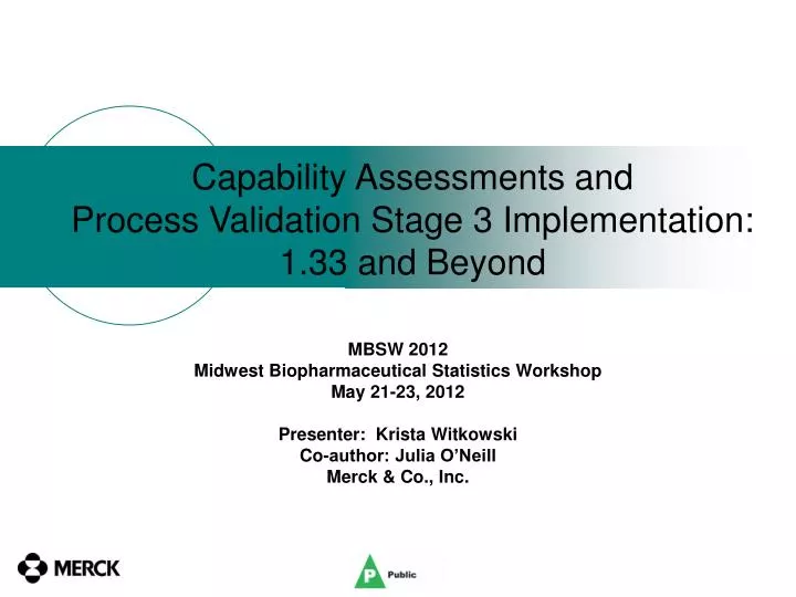
Capability Assessments and Process Validation Stage 3 Implementation: 1.33 and Beyond MBSW 2012 Midwest Biopharmaceutical Statistics Workshop May 21-23, 2012 Presenter: Krista Witkowski Co-author: Julia O’Neill Merck & Co., Inc.
Abstract This talk will discuss considerations for practitioners in pharmaceutical manufacturing as they implement the new FDA guidance for process validation. We will focus on Stage 3 - ongoing monitoring, or continued process verification - and how process capability is established, evaluated, and monitored. Examples on overcoming obstacles to implementation will be discussed, and the use of statistical thinking in our implementation strategy is highlighted.
Requirements of FDA Validation Guidance • FDA Guidance for Industry: Process Validation: General Principles and Practices, published January 2011 distinguishes three stages of validation: • Stage 1 – Process Design: The commercial manufacturing process is defined during this stage based on knowledge gained through development and scale-up activities. • Stage 2 – Process Qualification: During this stage, the process design is evaluated to determine if the process iscapable of reproducible commercial manufacturing. • Stage 3 – Continued Process Verification: Ongoing assurance is gained during routine production that the process remains in a state of control. • Further states that manufacturers should understandthe sources of variation • Detect the presence and degree of variation • Understand the impact of variation on the process and ultimately on product attributes • Control the variation in a manner commensurate with the risk it represents to the process and product
Process Validation Stage 2 Stage 1 Stage 3 Stage 3: Continued Process Verification
Stage 3: Continued Process Verification Goal=To continually assure that the process remains in a state of control (the validated state) during commercial manufacture.
Pharmaceutical Processes Autocorrelation Specifications based on process history Non-normal distributions common (e.g., lognormal) SPC Assumptions Independent results Specifications based on customer needs Normally distributed results Understanding Variation for Pharmaceutical Processes Issue: Statistical Process Control (SPC) procedures are generally designed based on assumptions not typically met by pharmaceutical processes:
Independent results Result vs. Previous Result – correlation not significant Autocorrelated results Result vs. Previous Result – significant correlation = .35 Issue 1: Autocorrelation
One Cause for Autocorrelation Production lots Propagation Purification Growth Production (Weeks) A new raw material lot introduced late in the production cycle has little opportunity to impact a product lot; however, a new raw material lot introduced early in the production cycle has a much greater opportunity to impact a product lot. This creates gradual trends (autocorrelation), rather than abrupt shifts, in product properties. Introduction of New raw material lot Introduction of New raw material lot
One Solution: Use long-term sigma Independent results: short-term and long-term limits are nearly equal. Long-term Short-term Autocorrelated results:short-term limits are narrowerthan long-term limits. Long-term limits are morerepresentative of process capability. Short-term Long-term
Example 2: Inherent mean shifts Mean shifts may be inherent – due to campaign effects, raw material changes, slight changes in processing conditions (e.g., seasonal effects). Short-term Long-term Results with mean shifts:short-term limits are narrowerthan long-term limits. Long-term limits are morerepresentative of process capability.
Understanding sources of variability Distribution of Variable A, with additional source of variability, µ=21.5, σ=2 Distribution of Variable A, with additional source of variability, µ=19, σ=2.5 Distribution of variable A reflecting initial sources of variability, µ=20, σ=2 Distribution reflecting all sources of variability Final limits (n=90) Early limits (n=30) Do not set limits too early, before all sources of variability are captured.
Statistical Thinking Strategy: for Autocorrelation • Standard Statistical Process Control (SPC) chart assumptions: • Observations are statistically independent – very important! • Observations are Normally distributed – much less important. • Limits are representative of expected performance. • Autocorrelation can have profound effects on the performance of SPC charts. • Considerations for control chart design: • Quickly signal real changes in results. • Reduce false alarms. • Make the chart easy to interpret – • present results in original scale, and • limits with a physical meaning. • Recommendation; • Set limits using the overall standard deviation based on a “long” stable period. • Bisgaard and Kulahci provide an elegant justification.
Issue 2: Establishing Process Capability • Two challenges: • Fundamental questions for pharmaceutical processes: • Are long-term shifts (for example, from raw material trends) “extraneous” sources of instability? • Or are they known and predictable special causes inherent to pharmaceutical process behavior? • Specifications may be set based on process consistency, not customer requirements.
Three Approaches to Capability Strategy Specification Spread Often underestimates total process variation Short-Term = 6 * short-term Sigma higher is better Specification Spread “Quality” = 6 * long-term Sigma Business Requirements “Business” = 6 * long-term Sigma
Well Off-target / Too Much Variation Relatively Close to Target / Moderate Variation Very Little Deviation From Target LSL USL LSL USL LSL USL Cpk < 1 Cpk = 1 Cpk > 1 Basics of Capability Calculations The mean and standard deviation are estimated from the centerline and control limits of the control charts, where three sigma is half the width of (UCL-LCL).
Grp 1 Grp 5 Grp 3 Grp 2 Grp 4 Short Term Studies Long Term Study Short term vs Long term
Example 2: Short term variability < Long term C indices underestimate total process variation when autocorrelation is present (when “within subgroup” variation is low compared to overall). Short-term Long-term Use the P-indices to provide a realistic assessment of long-term performance. For independent (not autocorrelated) processes, the P-indices and C-indices will be nearly equal. Cpk = 1.28 Ppk = 0.81
Example 2: Short term variability < Long term C indices underestimate total process variation when autocorrelation is present (when “within subgroup” variation is low compared to overall). Short-term Long-term Use the P-indices to provide a realistic assessment of long-term performance. For independent (not autocorrelated) processes, the P-indices and C-indices will be nearly equal. One-sided: USL = 1 Cpk = 1.28 Ppk = 0.81 Long-term Short-term
Risk Strategy: Ppk Comparison of CQA’s Capable & Stable Process (≥1.33) Process Robustness & Simplification Opportunities (<1.33) Frequency of monitoring report guided by risk strategy Ppk for 27 Critical Quality Attributes of a family of pharmaceutical products. Each bar represents the estimated Ppk for a single CQA. The bars are ordered from lowest Ppk (greatest risk) to highest. Note: Ppk is long-term capability, but takes into account centering of the process within specifications. In cases when there is a very large range of values for Ppk, a log scale can make this more read-able, while still maintaining the “red, yellow, green” risk categories
Z Score ZUPPER ZLOWER Other Choices in Capability Indicators Process Characterization Summary Statistics Indicators Cp Cpk Pp Ppk Gather Data Xbar (Mean) s (Std. Dev.) Proportion Defects OR Calculate Calculate using specifications and process data Use Z Table or Minitab Calculate Calculate Convert to DPM DPM(Upper) + DPM(Lower) = DPM (Total) Process Z Score Use Z Table or Minitab
USL- LSL 6 12 6 Cp = = Cp for a “6 sigma process”: = 2 Translating Pass/Fail to Ppk - type Index • Non-normal or pass/fail data: Use a "z-score" approach • Calculate the z-score using normal distribution theory • Proportion good z-score • Translate z-score to a “Ppk-type" scale: divide by 3. • Does not account for sample size, so results should be viewed in light of the amount of information you have • Example: • If 99% is "good“ (“within spec”): • z-score is 2.33, • Ppk = 2.33/3 = 0.78 3*Ppk = z-score Ppk = z-score / 3
Statistical Background on Capability • Capability index assesses whether a process is capable of meeting customer requirements. • Capability: “the natural or undisturbed performance after extraneous influences are eliminated” • from the Western Electric Company Statistical Quality Control Handbook (1956) • “Cpk can be calculated when the process is stable. Otherwise, for processes with known and predictable special causes and output meeting specifications Ppk should be used.” • from the AIAG PPAP Manual (2006) • Most important: PLOT THE DATA ON A CONTROL CHART. • Exact value of capability index is secondary.
Normal Results LogNormal Results Issue 3: LogNormally Distributed Results Error does not depend on measurement. Characterized by constant Standard Deviation. Results are symmetric within limits. Error is proportional to measurement. Characterized by constant Relative Standard Deviation (RSD) Results are not symmetric within limits. Has little impact if range of results is less than 10X. Easily corrected by analyzing results on the log scale.
LogNormal Results Log (LogNormal Results) Same data on different scale Solution: Log Transform Results Log transform makes error constant and results symmetric within limits.
References • Bisgaard, S., Kulahci, M.. (2005) Quality Quandaries: The Effect of Autocorrelation on Statistical Process Control Procedures. Quality Engineering 17: 481-489. • AIAG. “Definition of Process Measures.” Statistical Process Control. AIAG, 1995. pp 80-81. 2nd Printing. • The Black Belt Memory JoggerTM. (2002) GOAL/QPC Six Sigma Academy. First edition. p. 96.