Download
1 / 17
170 likes | 333 Views
MODELLING OF AIRFLOW OVER COMPLEX NATURAL LANDSCAPES. FOR EXPERIMENTAL DATA INTERPRETATION IN ENVIRONMENTAL RESEARCH. Sogachev Andrey 1 and Panferov Oleg 2. Contributors / Discussants:. Gennady Menzhulin, St. Petersburg Jon Lloyd, Jena Gode Gravenhorst, Göttingen Timo Vesala, Helsinki.

E N D
MODELLING OF AIRFLOW OVER COMPLEX NATURAL LANDSCAPES FOR EXPERIMENTAL DATA INTERPRETATION IN ENVIRONMENTAL RESEARCH Sogachev Andrey1 and Panferov Oleg2 Contributors / Discussants: Gennady Menzhulin, St. Petersburg Jon Lloyd, Jena Gode Gravenhorst, Göttingen Timo Vesala, Helsinki 1Division of Atmospheric Sciences, Department of Physical Sciences, University of Helsinki, POBox 64, FIN-00014, Helsinki, Finland (email: Andrei.Sogachev@helsinki.fi). 2Institute of Bioclimatology, University Göttingen, Büsgenweg 2, D-37077, Göttingen, Germany (email: opanfyo@gwdg.de)
The world-wide network of carbon flux measuring sites (total of 216 towers as of July 2003)
CO2 ? Interpretation of measurement data What part of the ecosystem does the flux sensor ‘see’ ? (Schmid, 2002, AFM)
Source weight function or flux footprint Definition In a simple form «footprint» or «source weight function» f (x,y,zm) is the transfer function between the measured value at a certain point F(0,0,zm) and the set of forcings on the surface-atmosphere interface F(x,y,0) (Schuepp et al., 1990, Schmid, 2002). (Schmid, 2002, AFM)
Model approaches for flux footprint estimation Eulerian analytic models (Schuepp et al.,1990; Horst and Weil, 1992) (zm, z0, d, u*, L) Lagrangian stochastic models(zm, z0, d, u*, L, TL, σu, σv, σw) Forward (pre-defined sources) (Leclerc et al., 1990; Wilson and Flesch, 1993)). Backward (pre-defined sensor location) (Flesch et al.,1995; Kljun et al., 1999). High tower Low tower (Schmid, 2002)
Approaches based on Navier-Stokes equations Most ecosystems are not spatially homogeneous. Linking the patch patterns to the carbon cycle is a serious challenge. Large-eddy simulation (Hadfield, 1994; Leclerc et al., 1997) Ensemble-averaged model (K-theory) (Sogachev et al., 2002)
F (CO2) Wind Z2m F (CO2) I Wind Z1m Z2m Z1m i = 1, 2, 3, k-2, k-1, k, I i = 1, 2, 3, k-2, k-1, k, I II III F (CO2) F (CO2) Wind Wind Z2m Z2m Z1m Z1m i = 1, 2, 3, k-2, k-1, k, I i = 1, 2, 3, k-2, k-1, k, I Methods of estimation of source weight function in ensemble-averaged model i indicates a model grid cell within a domain of I grid cells. k is the investigated grid cell (measurement point) . Z1 and Z2 are the heights for which the footprint is estimated. The dashed areas depict high intensity areas of vertical scalar flux. (Sogachev and Lloyd, 2004)
Upper boundary conditions +X V(t), Q ( t), T(t), q(t), C(t), U(t) f( x,y,z,t) +Y 0 -Y lateral borders -X 3 km 10 - 100 km ) Clouds ( t 10 - 100 m f = U, V, T , q , C, for x = ±X, y = ±Y c o n d i t i o n s o n 1 - 10 km T q F V = 0 U = 0 ( ( soil ), soil ), ( soil ), , advection CO2 l o w e r b o u n d a r y c o n d i t i o n s F E R H CO2 ¶ ¶ f f , ¶ ¶ x y G Scheme of the SCADIS (scalar distribution) model SCADIS is high resolution 3-D numerical model capable of computing the physical processes within both plant canopy and atmospheric boundary layer simultaneously. (Sogachev et al., 2002)
Basic characteristics of the SCADIS model • Terrain-following coordinate system • Basic equations: • momentum, • heat, • moisture, • scalars (CO2, SO2, O3), • turbulent kinetic energy (E) • One-and-a-half-order turbulence closure • based on equations of E and εor ω: E-l, E-ε, E-ω.) • Structure of vegetation • presented by type of vegetation • (vertical profile of LAD, leaf or needle size, • optical properties, aerodynamic drag coefficients …) • Vertical resolution • 75 - 110 model levels from • 0 to 3025 m, 42 of it between 0 and 35 m. (Sogachev et al., 2002; Sogachev et al., 2004, TAC)
Footprint and contribution function predicted by different methods Spatially homogeneous source located at a fixed height Effect of the vertical distribution of sources within a plant canopy Effect of φ=|Sc/S0| S0 is the soil respiration intensity; Sc is the photosynthetic activity of the canopy. (Sogachev and Lloyd, 2004)
Generalized effect of different disturbances on the airflow, scalar flux fields and the footprint (Sogachev et al., 2004, TAC)
N b 1 km 1. Effect of natural complex terrain on footprint Tver region, Russia a b (Sogachev and Lloyd., 2004)
2. Effect of natural complex terrain on footprint Hyytiälä, Finland (Sogachev et al., 2004, AFM)
N 100 m 3. Effect of natural complex terrain on footprint Solling, Germany (Sogachev et al., 2004, TAC)
Effect of forest edge on footprint Modelling aspects (Klaassen et al., 2002)
Tower To improve our understanding of the carbon cycle… Valkea-Kotinen Lake, Finland
Summary • Eddy covariance measuring system provide a piece of the C balance puzzle • The footprint of a turbulent flux measurement defines its spatial context. That is required for correct interpretation of experimental data. • Footprint models should produce realistic results in real-world situations • There are several methods to describe airflow (transported signal) in such situations by economical computing way with accuracy sufficient enough for practical tasks (K-l, K-ε, K-ω). • It has been demonstrated that they are suitable for footprint estimation. • Problems of airflow parameterization to be solved: • wake turbulence description within vegetation canopy remain uncertain. • (1-D verification is insufficient. It can lead to wrong conclusions). • soil (surface) flux description under condition of weak turbulence • flow separation within vegetation canopy: both for a dence forest on a flat • surface and for topography variations