Download
1 / 91
910 likes | 1.1k Views
Shading. Ming Ouhyoung 歐陽明 Professor Dept. of CSIE and GINM NTU. Illumination model. Ambient light ( 漫射 ) I = la * ka * Obj (r, g, b) la : intensity of ambient light ka : 0.0 ~ 1.0, Obj (r, g, b): object color Diffuse reflection ( 散射 )

E N D
Shading • Ming Ouhyoung • 歐陽明Professor • Dept. of CSIE and GINM • NTU
Illumination model • Ambient light (漫射) I = la * ka * Obj(r, g, b) la : intensity of ambient light ka : 0.0 ~ 1.0, Obj(r, g, b): object color • Diffuse reflection (散射) I = Ip (r, g, b) * Kd * Obj(r, g, b) * COS(theta-angle) Ip (r, g, b): light color • Light source attenuation
Specular reflection (似鏡面反射) • I = Ks * Ip(r, g, b) * COSn(alpha-angle), Ks = specular-reflection coef. • Phong illumination model color of object = Obj (R, G, B) = (Or, Og, Ob) or (light frequency) where 0.0 =< Od =< 1.0
Faster specular reflection calculation:Halfway vector approximation • halfway vector
Polygon shading : linear interpolation • flat shading : constant surface shading. • Gouraud shading: color interpolation shading. • Phong shading: vertex normal interpolation shading
Phong Shading • Use a big triangle, light shot in the center, as an example! • The function is really an approximation to Gaussian distribution macroscopic • The distribution of microfacets is Gaussian. [Torrance, 1967] (Beckmann distribution func.) • Given normal direction Na and Nb, Nm = ? • interpolation in world or screen coordinate? • in practice
Phong: under Ivan Sutherland • BùiTườngPhong (Vietnamese: BùiTườngPhong, December 14, 1942–1975) was a Vietnamese-born computer graphics researcher and pioneer. • He came to the University of UtahCollege of Engineering in September 1971 as a research assistant in Computer Science and he received his Ph.D. from the University of Utah in 1973. • Phong knew that he was terminally ill with leukemia while he was a student. In 1975, after his tenure at the University of Utah, Phong joined Stanford as a professor. He died not long after finishing his dissertation
What is the color of copper? • Reflection of copper • drastic change as a function of incidence angle [Cook, 82"]
New method: BRDF:Bi-directional Reflectance Density Function • Use a camera to get the reflection of materials from many angles • Light is also from many angles
BRDF • BRDF: a four-dimensional function that defines how light is reflected at an opaque surface. • The BRDF was first defined by Edward Nicodemus around 1965[1]. The modern definition is: F(ωi,ωo) = dL(ωo)/dE(ωi) = dL(ωo)/L(ωi)cos θidωi • where L is the radiance, E is the irradiance, and θi is the angle made between ωi and the surface normal, n.
BSSRDF • The Bidirectional Surface Scattering Reflectance Distribution Function (BSSRDF), is a further generalized 8-dimensional function S(Xi,ωi,Xo,ωo), in which light entering the surface may scatter internally and exit at another location. X describes a 2D location over an object's surface. • non-local scattering effects like shadowing, masking, interreflections or subsurface scattering.
SSBRDF, BSDF (Bidirectional scattering distribution function)
Homework #1 • Input : a file of polygons (triangles) • test image : a teapot, a tube • input format : Triangle fr, fg, fb, br, bg, bb x y z nxnynz x1, y1, z1, …. , ,X2, y2, z2 ……., /* where (fr, fg, fb) contains front face colors, (br, bg, bb) are background colors (x,y,z): 3D vertex position (nx,ny,nz) : vertex normal
Hw#1 requirements • Deadline Oct. 18 • Output: lines with colors • Rotation, Scaling, Translation, Shear • Clipping (front and back, left and right, top and bottom) • Camera: two different views • Object view and camera view • C, C++, Java, etc. • Limited open-GL library calls
Polygon file format used • e.q. Triangle frfgfbbrbg bb x1 y1 z1 nx1 ny1 nz1 x2 y2 z2 nx2 ny2 nz2 x3 y3 z3 nx3 ny3 nz3 Triangle • Where fr, fg, fb are foreground colors (Red Green Blue) nx, ny, nz are vertex normal
Other formats (more efficient) • Vertices 1, (x, y, z) 2, (x1, y1, z1) 3, … 23, … 890, …. 1010 • Triangle 1010, 23, 890 • Triangle 1, 2, 800
Visible-Surface Determination • The painter's algorithm • The Z-buffer algorithm • The point nearest to the eye is visible,..... • Very easy both for software and hardware. • Hardware Implementation: Parallel ---> fast display • Scan-line algorithms • One scan line at a time • Area-subdivision algorithm • Divide and conquer strategy • Visible-surface ray tracing
List-priority algorithms • Depth-sort algorithm sort by Z coord.(distance to the eye), resolve conflicts(splitting polygons), scan convert· ---v.s.---painter's algorithmBinary Space Partition • Trees(BSP tree)
The Display Order of Binary Space Partition Trees(BSP tree) if Viewer is in front of root, then • Begin {display back child, root, and front child} • BSP_displayTree(tree->backchild) • displayPolygon(Tree->root) • BSP_displayTree(tree->frontchild) • end else • Begin • BSP_displayTree(tree->frontchild) • displayPolygon(Tree->root) • BSP_displayTree(tree->backchild) • end
Visibility determination(2): Z-buffer algorithm Initialize a Z-buffer to infinity (depth_very_far) { Get a Triangle, calculate one point's depth from three vertices by linear interpolation If the one point's depth depth_P(x,y) is smaller than Z-Buffer(x,y) Z-Buffer (x,y) = depth_P(x,y), Color_at(x,y) = Color_of_P(x,y) else DO_NOTHING }
Homework #2 Shading • Scan convert the teapot which consists of triangles • Using Z-buffer algorithm for visible-surface determination • Flat, Gouraud shading and Phong shading, three light sources • Multiple lights, multiple 3D models (sphere, teapot, CSIE building etc)
HW#2: formula • Ia is object color • Ip is the color of light, and can have multiple lights • Note • color overflow problem (integer color up to 255) • MAX = max(R, G, B) = 255 etc. • Output format • RGBxRGBx.... 256*256 pixels • better results: 32<=R,G,B<=230, each 1 byte binary data
Visible line determination • Assume that visible surface determination can be done fast (by hardware Z-buffer or software BSP tree) • This method is used in most high performance systems now! • Depth cueing is more effective in showing 3D (in vector graphics machine, e.g. PS300). see sec. 14.3.4 • depth cueing: intensity interpolation
Visible - line determination: Appel's algorithm • quantitative invisibility of a point=0 --> visible • quantitative invisibility changes when it passes "contour line". • contour line:(define) • vertex traversing • EF: contour line • AB: whether this line segment is partially visible?
Standard Graphics Pipeline Ambient…and so on. 透視圖 著色 詳細
How to transform a plane? a surface normal? plane equation Ax + By + Cz + D = 0 NT*P=0 since p is transformed by M, How should we transform N? find Q, such that (Q*N)T*M*P=0 (N')T.(P')=0 i.e. NT*QT*M*P=0, i.e. QT*M=I ∴QT=M-1 Q=(M-1)T similar, the surface normal is transformed by Q, not M!!
Aliasing, anti-aliasing把一個pixel分成九塊九個中心,依照weighting來做blending
What is Volume Rendering? • The term volume rendering is used to describe techniques which allow the visualization of three-dimensional data. Volume rendering is a technique for visualizing sampled functions of three spatial dimensions by computing 2-D projections of a colored semitransparent volume.
There are many example images to be found which illustrate the capabilities of ray casting. These images were produced using IBM's Data Explorer Liver, Vessels
How to calculate surface normal for scalar field? • gradient vector • D(i, j, k) is the density at voxel(i, j, k) in slice k
Ray casting for volume rendering • Theory • Currently, most volume rendering that uses ray casting is based on the Blinn/Kajiya model. In this model we have a volume which has a density D(x,y,z), penetrated by a ray R.
Rays are cast from the eye to the voxel, and the values of C(X) and (X) are "combined" into single values to provide a final pixel intensity.
Transparency formula • For a single voxel along a ray, the standard transparency formula is: where: • Cout is the outgoing intensity/color for voxel X along the ray • Cinis the incoming intensity for the voxel • Splatting for transparent objects: back to front rendering • Eye Destination Voxel Source Voxel • Cd’= (1-αs) Cd +αs Cs αd’= (1-αs) αd + αs Cs : Color of source (background object color) αs: Opaque index (opaque = 1.0, transparency = 0.0) when background αs= 1.0, destination αd= 0.0, Cd’ = Cs, αd’ =αs, similarly, when foreground (destination) is NOT transparent, αd= 1.0, Cd’ = Cd(color of itself)
3D Modeling Methods • Creation of 3D objects • Revolving • 3D polygon • 3D mesh, 3D curves • Extrusion from 2D primitives (set elevation in Z-axis) • An example (new CS building construction)(step bye step demo) of AutoCAD • Feature that are useful • VPOINT, LIMITS, LINE, BREAK, Elevation, SNAP, GRID, etc • 3D digitizers
Texture mapping 1. What is texture? 2. How to map a texture to an object surface? <- : direction of mapping pixel value = sum of weighted texels within the four corners mapped from a pixel 3. See pictures
Curves and surfaces • Used in airplanes, cars, boats • Patch (補片)
How to model a teapot? • How to get all the triangles for a teapot? • What kind of curved surfaces? • How to display (scan convert) these surfaces? • What's the surface normal? • Discuss ways to "define" a curved surfaces. • Can we show an implicit surface equation easily? • e.g. f(x,yx,z) = ax2 + by2 + cz2 + 2dxy + 2eyz + 2fxz + 2gx + 2hy + 2jz + k = 0 • Given (x,y), find z value • Double roots, no real roots?
Curves and Surfaces • Topics • Polygon meshes • Parametric cubic curves • Parametric bicubic surfaces • Quadric surfaces Parametric cubic curves x(t) = axt3 + bxt2 + cxt + dx y(t) = ayt3 + byt2 + cyt + dy z(t) = azt3 + bzt2 + czt + dz • Continuity conditions • Geometric continuity (G0): join together • Parametric continuity (C1) (see below) • Cncontinuity: dn / dtn[Q(t)]continuous
B'ezier Curve Q'(0) = 3 (p1-p0) Q'(1) = 3 (p3-p2) Why choosing "3" ? Q(t) = (1-t)3p0 + 3t(1-t)2p1 + 3t2(1-t)p2 + t3p3 ............e.q.11.29
Bezier curve(2) in matrix form T*MB*GB Note: Q'(0) = -3(1-t)2p0 + 3(1-t)2p1|t=0 =3(p1-p0) if p1 - p4 is equally spaced, the curve Q(t) has constant velocity! (that's why to choose 3)
Subdividing B'ezier curves Advantage of B'ezier curves • explicit control of tangent vectors-->interactive design • easy subdivision-->decompose into flat (line) segments
Subdividing B'ezier curves(2) • new control points: pa, pb, pc, pe, pf, • in addition to p1, p2, p3, p4