Download

1 / 25
250 likes | 257 Views
Quadratic Solvability. The P C P starting point. Overview. In this lecture we’ll present the Quadratic Solvability problem. We’ll see this problem is closely related to PCP . And even use it to prove a (very very weak...) PCP characterization of NP. Example: =Z 2 ; D=1 y = 0

E N D
Quadratic Solvability The PCP starting point
Overview • In this lecture we’ll present the Quadratic Solvability problem. • We’ll see this problem is closely related to PCP. • And even use it to prove a (very very weak...) PCP characterization of NP.
Example: =Z2; D=1 y = 0 x2 + x = 0 x2 + 1 = 0 Quadratic Solvability or equally: a set of dimension D total-degree 2 polynomials Definition (QS[D, ]): Instance: a set of n quadratic equations over with at most D variables each. Problem: to find if there is a common solution. 0 1 1 1
Solvability A generalization of this problem is the following: Definition (Solvability[D, ]): Instance: a set of n polynomials over with at most D variables. Each polynomial has degree-bound n in each one of the variables. Problem: to find if there is a common root.
Solvability is Reducible to QS: Proof Idea w2 w2 y2 x2 + x2 t + tlz + z + 1 = 0 w3 w1 w1 = y2 w2 = x2 w3 = tl the parameters (D,) don’t change (assuming D>2)! Could we use the same “trick” to show Solvability is reducible to Linear Solvability?
3-SAT For completeness we provide the definition of 3-SAT: Definition (3-SAT): Instance: a 3CNF formula. Problem: to decide if this formula is satisfiable. (123)...(m/3-2m/3-1m/3) where each literal i{xj,xj}1jn It is well known that 3-SAT is NP-Complete.
3-SAT is Reducible to Solvability Given an instance of 3-SAT, use the following transformation on each clause: Tr[ xi ] = 1 - xi Tr[ xi ] = xi Tr[ ( i i+1 i+2 ) ] = Tr[ i ] * Tr[ i+1 ] * Tr[ i+2 ] The corresponding instance of Solvability is the set of all resulting polynomials. For the time being, assume the variables are only assigned {0,1}
3-SAT is Reducible to Solvability: Removing the Assumption In order to remove the assumption we need to add the equation xi * ( 1 - xi ) = 0 for every variable xi. This concludes the description of a reduction from 3SAT to Solvability[O(1),] for any field . What is the maximal dependency?
QS is NP-hard Proof: by the two above reductions. 3-SAT Solvability QS
Arithmization • To translate 3-SAT to Solvability we used the idea of aritmization. • The simple trick is widely used in PCP proofs, as well as in other fields.
Gap-QS Definition (Gap-QS[D, ,]): Instance: a set of n quadratic equations over with at most D variables each. Problem: to distinguish between: There is a common solution No more than an fraction of the equations can be satisfied simultaneously. YES NO
Gap-QS and PCP the variables of the input system Gap-QS[D,,] Reminder: LPCP[D,V, ] if there is an efficient algorithm, which for any input x, producesa set of efficient Boolean functions over variables of range 2V,each depending on at mostD variables. xL iff there exits an assignment to the variables, which satisfies all the functions xL iff no assignment can satisfy more than an -fraction of the functions. Gap-QS[D,,] PCP[D,log||,] quadratic equations system For each quadratic polynomial pi(x1,...,xD), add the Boolean function i(a1,...,aD)pi(a1,...,aD)=0 values in
Proving PCP Characterizations of NP through Gap-QS • Therefore, every language which is efficiently reducible to Gap-QS[D,,]is also in PCP[D,log||,]. • Thus, proving Gap-QS[D,,] is NP-hard, also proves the PCP[D,log||,] characterization of NP. • And indeed our goal henceforth will be proving Gap-QS[D, ,] is NP-hard for the best D, and we can.
degree-2 polynomials p1 p2 p3 . . . pn i 650 . . . 0 any assignment Some Gap-QS is NP-hard Proof: by reduction from QS[O(1),]. Proof Idea: Observe an instance of QS[O(1),]: we need an efficientdegree-preserving transformation on the polynomials which induces a trans. E on the evaluations s.t.: 1) E(0n)=0m 2) v0n, (E(v),0m) is big. there might be a lot of zeroes p1’p2’p3’. . . pm’ not many zeroes 024 . . . 3
c1 . . . cm p p1 p2 ... pn c11 . . . c1m . . . . . . . . . cn1 . . .cnm p•c1 . . . p•cm = Multiplication by a Matrix Preserves the Degree polynomials poly-time, if m=nc inner product a linear combination of polynomials scalars
c1 . . . cm e1 e2 ... en c11 . . . c1m . . . . . . . . . cn1 . . .cnm •c1 . . . •cm = How Does a Multiplication Affect the Evaluations Vector? the values of the polynomials under some assignment the values of the new polynomials under the same assignment a zero vector if =0n
Suitable Matrices • A matrix Anxm which satisfies for every vu,(vA,uA)1- is a linear code. • Note, that this is completely equivalent to saying Anxm satisfies for every v0n,(vA,0m)1-. • That’s because (vA,uA)=((v-u)A,0m).
What’s Ahead • We proceed with several examples for linear codes: • Reed-Solomon code • Random matrix • And finally even a code which suits our needs... the “generic -code” from the Encodings lecture.
Using Reed-Solomon Codes • Define the matrix as follows: That’s really Lagrange’s formula in disguise... • One can prove that for any 0i||-1, (vA)i is P(i), where P is the unique degree n-1 univariate polynomial, for which P(i)=vi for all 0in-1. • Therefore for any v the fraction of zeroes in vA is bounded by (n-1)/||. using multivariate polynomials we can even get =O(logn/||)
for any 1||-1 A Random Matrix Should Do Lemma: A random matrix Anxm satisfies w.h.p. v0nn,|{i : (vA)i = 0}| / m < 2||-1 Proof: Let v0nn. • 1im PrAnxm[ (vA)i = 0 ] = ||-1 The inner product of v and a random vector is random. • |{i : (vA)i = 0}| (denoted Xv) is a binomial r.v with parameters m and ||-1. • By the Chernoff bound, Pr[ Xv 2m||-1 ] 2e-m/4||.
A Random Matrix Should Do Every v0n disqualifies at most 2e-m/4|| of the matrices nxm At most 2||ne-m/4|| of the matrices are disqualified That is, Pr[ v0n: Xv/m 2||-1 ] 2||ne-m/4||. For m=O(n||log||), the claim holds.
p2k pk-1 Deterministic Construction Assume =Zp. Let k=logpn+1. (Assume w.l.o.g kN) Let Zpk be the dimension k extension field of . associate each column with a pair(x,y)ZpkZpk associate each row with 1ipk-1 <xi,y>
Analysis degree-pk-1 polynomial, denoted G(x) • For any vn, for any (x,y)ZpkZpk, • The number of zeroes in vA where v0n x,y: G(x)=0 + x,y: G(x)0 <G(x),y>=0 • And thus the fraction of zeroes
Summary of the Reduction Given an instance {p1,...,pn} for QS[O(1),], find a matrix A which satisfies v0n|{i : (vA)i = 0}| /m < 2||-1 {p1,...,pn} QS[O(1),] iff {p1A,...,pnA} Gap-QS[O(n),,2||-1] !!
Hitting the Road This proves a PCP characterization with D=O(n) (hardly a “local” test...). Eventually we’ll prove a characterization with D=O(1) ([DFKRS]) using the results presented here as our starting point.