Rad ial Basis Networks

1. Radial Basis Networks

2. Introduction • Radial basis networks may require more neurons than standard feed-forward backpropagation networks, but often they can be designed in a fraction of the time it takes to train standard feed-forward networks. They work best when many training vectors are available.

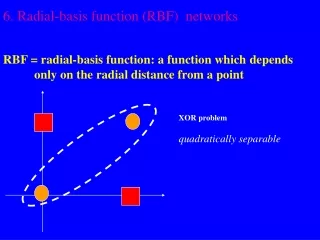
3. Radial Basis Functions • Net input to the radbas transfer function is the vector distance between its weight vector w and the input vector p, multiplied by the bias b. • The radial basis function has a maximum of 1 when its input is 0. As the distance between w and p decreases, the output increases. Thus, a radial basis neuron acts as a detector that produces 1 whenever the input p is identical to its weight vector p.

4. Continue • The bias b allows the sensitivity of the radbas neuron to be adjusted. For example, if a neuron had a bias of 0.1 it would output 0.5 for any input vector p at vector distance of 8.326 (0.8326/b) from its weight vector w.

5. Network Arhitecture • Radial basis networks consist of two layers: a hidden radial basis layer of S1 neurons, and an output linear layer of S2 neurons.

6. Continue • We can understand how this network behaves by following an input vector p through the network to the output a2. If we present an input vector to such a network, each neuron in the radial basis layer will output a value according to how close the input vector is to each neuron's weight vector.

7. Continue • Thus, radial basis neurons with weight vectors quite different from the input vector p have outputs near zero. These small outputs have only a negligible effect on the linear output neurons. • In contrast, a radial basis neuron with a weight vector close to the input vector p produces a value near 1. If a neuron has an output of 1 its output weights in the second layer pass their values to the linear neurons in the second layer.

8. Continue • In fact, if only one radial basis neuron had an output of 1, and all others had outputs of 0's (or very close to 0), the output of the linear layer would be the active neuron's output weights. This would, however, be an extreme case. Typically several neurons are always firing, to varying degrees.

9. Probabilistic Neural Network • Probabilistic neural networks can be used for classification problems. When an input is presented, the first layer computes distances from the input vector to the training input vectors, and produces a vector whose elements indicate how close the input is to a training input. The second layer sums these contributions for each class of inputs to produce as its net output a vector of probabilities.

10. Continue • Finally, a compete transfer function on the output of the second layer picks the maximum of these probabilities, and produces a 1 for that class and a 0 for the other classes.

11. Example • P = [0 0;1 1;0 3;1 4;3 1;4 1;4 3]‘; • Tc = [1 1 2 2 3 3 3]; • We need a target matrix with 1's in the right place. We can get it with the function ind2vec. It gives a matrix with 0's except at the correct spots. So execute • T = ind2vec(Tc)

12. Continue • plot(P(1,:),P(2,:),'.','markersize',30) • for i=1:7, text(P(1,i)+0.1,P(2,i),sprintf('class %g',Tc(i))), end • axis([-5 5 -5 5]) • net = newpnn(P,T);

13. Testing • P2 = [1 4;0 1;5 2]‘; • a = sim(net,P2); • ac = vec2ind(a); • plot(P2(1,:),P2(2,:),'.','markersize',30,'color',[1 0 0]) • for i=1:3, text(P2(1,i)+0.1,P2(2,i),sprintf('class %g',ac(i))), end • axis([-5 5 -5 5])

14. Conclusion • Radial basis networks can be designed very quickly • Probabilistic neural networks (PNN) can be used for classification problems. Their design is straightforward and does not depend on training. A PNN is guaranteed to converge to a Bayesian classifier providing it is given enough training data. These networks generalize well.

15. Continue • But, they are slower to operate because they use more computation than other kinds of networks to do their function approximation or classification.