Download

1 / 79
790 likes | 794 Views
Discover the fascinating world of fractals, self-similar mathematical objects, through the MegaMenger project. Explore the Cantor Set, Sierpinski Carpet, and Menger Sponge, and learn how to create discrete models of these fractals. Join the global effort to construct 20 level 3 models of the Menger Sponge using business cards.

E N D
MegaMenger Graphs Allan Bickle Calvin College MegaMenger Graphs
Fractals • A fractal is a type of mathematical object. • Many well-known fractals are self-similar. That is, part of the object is isomorphic to the whole. • Often, a fractal can be formed by iterating some operation infinitely many times on a set.
The Cantor Set • For example, consider the Cantor set. Begin with the interval [0,1] and remove the middle third. This leaves the set which contains two intervals of length 1/3. Next, remove the middle thirds of both of these subintervals. • At each step, remove the middle third of each subinterval remaining. Iterating this operation infinitely many times produces the Cantor set.
The Cantor Set • Note that the portion of the Cantor set in is isomorphic to the entire set. • Here we see levels 0-5 of the construction of the Cantor Set.
The Sierpinski Carpet • The Cantor set is a subset of a line, which is one-dimensional. We can generalize it to higher dimensional fractals. • One way of doing this is to start with a square, divide it into nine smaller equal-sized squares, and remove the middle square. Then repeat the operation on each smaller square ad infinitum. • This produces a fractal called the Sierpinski carpet. This can be seen to contain many copies of the Cantor set.
The Menger Sponge • One way of generalizing this idea to a three dimensional object is to start with a cube, and divide it into 27 smaller equal-sized cubes. Then remove the middle cube from each face and the center cube, leaving 20 smaller cubes. Then repeat the operation on each smaller cube ad infinitum. • This produces a fractal called the Menger sponge. This can be seen to contain many copies of the Sierpinski carpet. • It was first described in 1926 by Karl Menger, who is famous in graph theory for Menger's Theorem on connectivity.
Discrete Models of Fractals • If we want to build real world models of these fractals, we cannot perform infinitely many iterations of an operation. Even performing finitely many operations eventually becomes impossible if it requires us to remove smaller and smaller portions of a real world object. • An alternative way to construct real world models of fractals is to start with a given unit and build larger and larger models out of more and more copies of this unit. We will refer to these as levels of the fractal model.
Discrete Models of Fractals • Thus level 0 for the Sierpinski carpet is a square, and level 1 is built by arranging eight of these squares into a ring. Then level 2 is built by arranging eight copies of level 1 into a ring, and so on. • For the Menger sponge, level 0 is a cube, and level 1 is built out of twenty of these cubes. Level two is built out of twenty copies of level 1, and so on.
Discrete Models of Fractals • We would like a way to describe the locations of the level 0 units in these constructions. To describe the location of a subinterval in the Cantor set, label it 0, 1, or 2 depending which third of the interval it is contained in. Then append a 0, 1, or 2 for which third of this subinterval it is contained in. • Continuing in this fashion, we obtain a string of 0's, 1's, and 2's that describes the location of the subinterval. But if the subinterval is actually in the Cantor set, 1 cannot appear. • We can think of such a string of length i as a ternary number between 0 and 3i -1 describing the location of a subinterval in level i of the model of the Cantor set. • For example, 0220 represents 270+92+32+10=90.
Discrete Models of Fractals • Since the Sierpinski carpet is a subset of the plane, we assign two coordinates to indicate the location of a square in it. • Each coordinate is described by a ternary string constructed analogously to that for the Cantor set. • A square is contained in the Sierpinski carpet if and only if its coordinates do not both contain a 1 in the same position.
Discrete Models of Fractals • For the Menger sponge, we assign three coordinates to indicate the location of a cube in it. Each coordinate is described by a ternary string constructed analogously to that for the Cantor set. • A cube is contained in the Menger sponge if and only if there is at most one 1 in any position of its three coordinates. • For example, (10,01,02) is in the Menger sponge, but (10,01,12) is not.
The MegaMenger Project • The goal of the MegaMenger project was to build twenty level 3 models of the Menger sponge out of business cards at sites around the world. • Each level one cube was constructed out of six cards, and has side length two inches with two flaps on each face that were used for linking it with other cubes. • Once all the cubes were linked together, another card was attached to each face to hide the exposed flaps, add aesthetic appeal, and provide additional structural support. • The level 3 model has side length 4.5 feet and weighs approximately 170 pounds.
The MegaMenger Project • The MegaMenger project was organized by Queen Mary University of London. I participated in Calvin College's project, which was organized by Randy Pruim and Gerard Venema and took place during October 2014. • More information is available at http://www.megamenger.com/ and http://www.calvin.edu/academics/departments-programs/mathematics-statistics/mega-menger/. • Following are some photos that illustrate the process.
Graph Theory Models • This project inspired me to ask and answer a number of questions about models of the Sierpinski carpet and Menger sponge. • We will use graph theory to model the real world models of the Sierpinski carpet and Menger sponge. • A graph is composed of a set of vertices and a set of edges, which is a subset of the set of 2-element subsets of the vertex set. • In a Sierpinski carpet graph, each vertex represents a square of the carpet. Vertices are adjacent if their squares share a common edge.
Graph Theory Models • In a Menger sponge graph, each vertex represents a cube of the sponge. Vertices are adjacent if their cubes share a common face. • We will denote the level i Sierpinski carpet graph as SCi, and the level i Menger sponge graph as MSi. • We will use graph theory to find information about the structure of the Sierpinski carpets and Menger sponges. We begin by calculating some parameters of these graphs.
Orders of the Graphs • The order of a graph, n(G), is the number of vertices in graph G. • Each iteration in the construction of the Cantor set can be formed from two copies of the previous one. This gives us the recurrence relation for the number of intervals ci = 2ci-1, with initial condition c0 = 1. • This immediately gives the exponential solution ci = 2i.
Orders of the Graphs • The Sierpinski carpet is formed from eight copies of the previous level, so the order n(SCi) = 8·n(SCi-1) and n(SC0) = 1. Thus n(SCi) = 8i. • The Menger sponge is formed from twenty copies of the previous level, so n(MSi) = 20·n(MSi-1) and n(MS0) = 1. Thus n(MSi) = 20i.
Sizes of the Sierpinski Carpets • The size m(G) of a graph is the number of edges it contains. • To determine the sizes of the Sierpinski carpet graphs, we must develop a recurrence relation. • Obviously, m(SC0) = 0 and m(SC1) = 8. • Each level is formed from eight copies of the previous level with some added edges in between.
Sizes of the Sierpinski Carpets • There are 3i-1 edges between each copy of SCi. Since there are eight edges in SC1, there are eight sets of 3i-1 edges added. Thus we find the recurrence relation m(SCi) = 8·m(SCi-1)+8·3i-1. • This is a nonhomogeneous linear recurrence relation. The homogeneous part is exponential, so it has a solution of the form A8i. • A theorem on recurrence relations tells us that the nonhomogeneous part has a solution of the form B3i.
Sizes of the Sierpinski Carpets • Thus the solution should have the form m(SCi) = A8i + B3i. • Plugging in the initial conditions, we find 0 = A + B and 8 = 8A + 3B. • Solving this system of linear equations, we find A = 8/5 and B = -8/5 . Thus m(SCi) = (8/5)8i – (8/5)3i. • The first few terms of this sequence are 0, 8, 88, 776, 6424, ... • This also implies that the average degree of the Sierpinski carpet graphs approaches 16/5 = 3.2 as i grows large.
Sizes of Menger Sponge Graphs • To determine the sizes of the Menger sponge graphs, we use a similar method. • We see m(MS0) = 0 and m(MS1) = 24. • Each level is formed from 20 copies of the previous level with some added edges in between. There are 8i-1 edges between each copy of MSi, since each face of the Menger sponge is a level i-1 Sierpinski carpet. Since there are 24 edges in MS1, there are 24 sets of 8i-1 edges added. • Thus we find the recurrence relation m(MSi) = 20·m(MSi-1)+24·8i-1.
Sizes of Menger Sponge Graphs • The homogeneous part is exponential, so it has a solution of the form A20i. The nonhomogeneous part has a solution of the form B8i. Thus the solution should have the form m(MSi) = A20i+B8i. • Plugging in the initial conditions, we find 0 = A + B and 24 = 20A + 8B. Solving this system of linear equations, we find A = 2 and B = -2. Thus m(MSi) = 2·20i-2·8i. • The first few terms of this sequence are 0, 24, 672, 14976, 311808, ... • This also implies that the average degree of the Menger sponge graphs approaches 4 as i grows large.
Surface Area of Menger Sponges • In constructing a model of the Menger sponge, we added extra cards on the outside faces to improve its aesthetics and stability. • To determine how many cards were needed, we want to find the surface area of the Menger sponge. • When constructing a level from the twenty copies, we see that some outside faces will be covered up. • Thus it is convenient to split the surface area into the inside surface area and outside surface area.
Surface Area of Menger Sponges • For the inside surface area, we note that IS (MS1) = 24, since each of the twelve cubes of degree two has two interior faces. • Now level i is composed of twenty copies of level i-1. In addition, there are 24 inside faces that are level i-1 Sierpinski carpets. • Thus we find the recurrence relation IS(MSi) = 20·IS(MSi-1)+24·8i-1.
Surface Area of Menger Sponges • This is the same recurrence relation as for the size of the Menger sponge! • It also has the same initial condition, so it has the same solution, IS(MSi) = 2·20i-2·8i. • One way of illustrating the relationship between the size and inside surface area is to note that in the level one cube, each vertex of degree two is incident with two edges (and this counts all the edges exactly once) and the corresponding cube has two inside faces.
Surface Area of Menger Sponges • For the outside surface area, we note that there are six outside faces. Each face is a level i Sierpinski carpet, which has order 8i. Thus the outside surface area is 6·8i. • Adding the inside and outside surface areas, we see that the total surface area of MSi is 2·20i+4·8i. • The first few terms of this sequence are 6, 72, 1056, 18048, 336384, ...
Partite Sets of Menger Sponges • Calculating the chromatic number of the Sierpinski carpet and Menger sponge graphs is not an interesting problem since these graphs are easily seen to be bipartite. • A more interesting problem is determining the cardinalities of the two partite sets. • First we note that all of the corners of any Menger sponge graph are in the same partite set since any two corners are an even distance apart. • We denote the cardinality of this partite set as n’i, and the cardinality of the other partite set as n"i. • We see that n’0 = 1, n"0 = 0, n’1 = 8, and n"1 = 12.
Partite Sets of Menger Sponges • When we construct level i, set n’i consists of the sets n’i-1 for the corner level i-1 cubes of level i, and also contains the sets n"i-1 of the non-corner level i-1 cubes of level i. • Thus some of the sets 'switch places', so the recurrences for each partite set depend on both. • Specifically, we find n’i = 8n’i-1+12n"i-1 and n"i = 12n’i-1+8n"i-1. We can write this in matrix form.
Partite Sets of Menger Sponges • To solve this discrete dynamical system, we find the eigenvalues of the coefficient matrix A. • We see det(A-λI) = (8-λ)2-122 = λ2-16λ-80 = (λ-20)(λ+4), so the eigenvalues are λ1 = 20 and λ2 = -4. • For λ1, we see A-λ1I = , so the corresponding eigenvector is v1 = (1,1). • For λ2, we see A-λ2I = , so the corresponding eigenvector is v2 = (1,-1).
Partite Sets of Menger Sponges • It is known in linear algebra that (n’i,n"i) = A(λ1)iv1+B(λ2)iv2. We plug in the initial conditions, finding • It is easy to see that A = 1/2 , B = 1/2 is the solution. Thus we find that n’i = (1/2)20i + (1/2)(-4)i and n"i = (1/2)20i –(1/2)(-4)i. Notably, which set is larger alternates between successive levels. • The first few terms of the sequence for n’ are 1, 8, 208, 3968, 80128, ... and the first few terms of the sequence for n" are 0, 12, 192, 4032, 79872, ...
Vertex Degrees in Sierpinski Carpets • The degree of a vertex is the number of edges incident with it. • Examining the vertices of the Sierpinski carpet graphs, we find vertices of degree two, three, and four. How many are there of each? • We denote by d2k(i) the number of vertices of degree k in SCi. • We note that SC1 has eight vertices of degree two and none of degree three or four. • Each level i Sierpinski carpet is formed from eight copies of level i-1 with eight sets of 3i-1 edges added in between.
Vertex Degrees in Sierpinski Carpets • We refer to the set of vertices for which one of the dimensions is as large (or small) as possible as a boundary of the carpet. • Each set of edges added between level i-1 carpets will increase the degrees of the vertices in two boundary sets. Thus we must add in or subtract out the vertices in these 16 boundary sets to count the vertices of a particular degree correctly. • In addition, there are four vertices contained in two boundary sets, so we must also make sure that these vertices are counted correctly.
Vertex Degrees in Sierpinski Carpets • We need to know the degrees of the vertices in the boundary sets of a level i carpet. • For level 1, we have three vertices of degree two. To construct the next level, we take three copies of this side, which makes four vertices of degree three. • Let d12(i) be the number of vertices of degree two in the boundary of the level i Sierpinski carpet and d13(i) be the number of vertices of degree three.