Download
1 / 55
550 likes | 560 Views
Least Squares Regression. Fitting a Line to Bivariate Data. Automating Least Squares Line and Related Calculations. Excel: In text: see p. 200-201

E N D
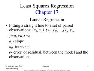
Least Squares Regression Fitting a Line to Bivariate Data
Automating Least Squares Line and Related Calculations • Excel: • In text: see p. 200-201 • Excel has extensive capabilities related to least squares lines; in the Excel help search line type terms such as: slope, intercept, trendline, and regression for more information. • Statcrunch • In the left panel of our class webpage http://www.stat.ncsu.edu/people/reiland/courses/st311/ click on Student Resources, in “Statcrunch Instructional Videos” see “Scatterplots and Regression”; in “Many Statcrunch Instructional Videos” see videos 16, 19, 24, 48, and 48 (these numbers may change as more videos are added to this YouTube site). • TI calculator: • In the left panel of our class webpage click on Student Resources; under “Graphing Calculators, Online Calculations”, either • click on TI Graphing Calculator Guide and see p. 7-9, or • click on Online Graphing Calculator Tutorials
Avg. occupants per car 1980: 6/car 1990: 3/car 2000: 1.5/car By the year 2010 every fourth car will have nobody in it! Food for Thought Kind of mathematical relationship between year and avg. no. of occupants per car? Why might relation- ship break down by 2010? Linear Relationships
Basic Terminology • Scatterplots, correlation: interested in association between 2 variables (assign x and y arbitrarily) • Least squares regression: does one quantitative variable explain or cause changes in another variable?
Basic Terminology (cont.) • Explanatory variable: explains or causes changes in the other variable; the x variable. (independent variable) • Response variable: the y -variable; it responds to changes in the x - variable. (dependent variable)
Examples • Fertilizer (x ) corn yield (y ) • Advertising $ (x ) store income (y ) • Drug dose (x ) blood pressure (y ) • Daily temperature (x ) natural gas demand (y ) • change in min wage(x) unemployment rate (y)
Simplest Relationship • Simplest equation that describes the dependence of variable y on variable x y = b0 + b1x • linear equation • graph is line with slope b1 and y-intercept b0
Graph y=b0 +b1x y rise Slope b=rise/run b0 run 0 x
Notation • (x1, y1), (x2, y2), . . . , (xn, yn) • draw the line y= b0 + b1x through the scatterplot , the point on the line corresponding to xi is
Observed y, Predicted y predicted y when x=2.7 yhat = a + bx = a + b*2.7 2.7
Scatterplot: Fuel Consumption vs Car Weight “Best” line?
Criterion for choosing what line to draw: method of least squares • The method of least squares chooses the line that makes the sum of squares of the residuals as small as possible • This line has slope b1 and intercept b0 that minimizes
Questions • Construct scatterplot; determine if linear model is appropriate. If so … • … find the least squares prediction line • Estimate consumption expenditure in a household with an income of (i) $6,000 (ii) $25,000. Comfortable with estimates? • Compute the residuals
The least squares line always goes through the point with coordinates (x, y) ( x, y ) = ( 9, 8 )
Sresiduals, S(residuals)2 • Note that • Sresiduals = 0 • S(residuals)2 = 3.6 • From formula on slide 15: SSE=yi2 – b0*yi – b1*xiyi 330 – 6.2*40 - .2*392 = 330 – 248 – 78.4 = 3.6 Any other line drawn through the scatterplot will have S(residuals)2 > 3.6
Car Weight, Fuel Consumption Example, cont. (xi, yi): (3.4, 5.5) (3.8, 5.9) (4.1, 6.5) (2.2, 3.3) (2.6, 3.6) (2.9, 4.6) (2, 2.9) (2.7, 3.6) (1.9, 3.1) (3.4, 4.9)
The Least Squares Line Always goes Through ( x, y ) (x, y ) = (2.9, 4.39)
Using the least squares line for prediction. Fuel consumption of 3,000 lb car? (x=3)
Be Careful! Fuel consumption of 500 lb car? (x = .5) x = .5 is outside the range of the x-data that we used to determine the least squares line
Avoid GIGO! Evaluating the least squares line • Create scatterplot. Approximately linear? • Calculate r2, the square of the correlation coefficient • Examine residual plot
r2 : The Variation Accounted For • The square of the correlation coefficient r gives important information about the usefulness of the least squares line
r2: important information for evaluating the usefulness of the least squares line -1 ≤ r ≤ 1 implies 0 ≤ r2 ≤ 1 The square of the correlation coefficient, r2, is the fraction of the variation in y that is explained by the least squares regression of y on x. The square of the correlation coefficient, r2, is the fraction of the variation in y that is explained by the variation in x.
Example: car weight, fuel consumption • x=car weight, y=fuel consumption r2 = (.9766)2 .95 About 95% of the variation in fuel consumption (y) is explained by the linear relationship between car weight (x) and fuel consumption (y). • What else affects fuel consumption? • Driver, size of engine, tires, road, etc.
SAT scores: result r2 = (-.868)2 = .7534 If 57% of NC seniors take the SAT, the predicted mean score is
Avoid GIGO! Evaluating the least squares line • Create scatterplot. Approximately linear? • Calculate r2, the square of the correlation coefficient • Examine residual plot
Residuals • residual =observed y - predicted y = y - y • Properties of residuals • The residuals always sum to 0 (therefore the mean of the residuals is 0) • The least squares line always goes through the point (x, y)
Graphicallyresidual = y - y y yi yi ei=yi - yi X xi
Residual Plot • Residuals help us determine if fitting a least squares line to the data makes sense • When a least squares line is appropriate, it should model the underlying relationship; nothing interesting should be left behind • We make a scatterplot of the residuals in the hope of finding… NOTHING!
Car Wt/ Fuel Consump: Residuals • CAR WT. FUEL CONSUMP. Pred FUEL CONSUMP. Residuals • 3.4 5.5 5.2094980690 .290501931 • 3.8 5.9 5.865096525 0.034903475 • 4.1 6.5 6.356795367 0.143204633 • 2.2 3.3 3.242702703 0.057297297 • 2.6 3.6 3.898301158 -0.29830115 • 2.9 4.6 4.39 0.21 • 2 2.9 2.914903475 -0.01490347 • 2.7 3.6 4.062200772 -0.46220077 • 1.9 3.1 2.751003861 0.348996139 • 3.4 4.9 5.209498069 -0.309498069