Download
1 / 36
370 likes | 483 Views
Varieties of Causal Sets. Jose L Balduz Jr Department of Physics Mercer University APS Meeting April 2007. Outline: Varieties of Causal Sets. What Are Causal Sets? Why? Standard definition (partial ordering). Motivation. Allowed structures in standard causal sets.

E N D
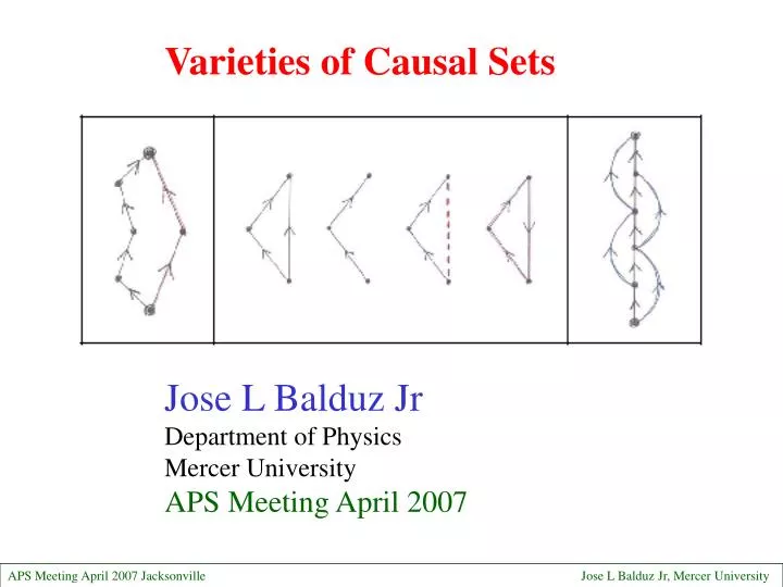
Varieties of Causal Sets Jose L Balduz Jr Department of Physics Mercer University APS Meeting April 2007
Outline: Varieties of Causal Sets • What Are Causal Sets? Why?Standard definition (partial ordering). Motivation. Allowed structures in standard causal sets. • Generalized Causal SetsTransitive link as physical nonlocal connection. Geodesic core and halo. Time dilation. Missing link, spacelike link, causal loop link. • Spacelike LinksGenerating causal sets from hypergraphs. Allowed structures. Duality. Time and distance measures; the light cone. • Causal LoopsThe (forward and backward) Global Ordering. Construction. Invariant skeleton. Loops and their causal shadows. • Nonlocal LinksA conductance model for effective distance, with probabilitistic halo. Distance shrinkage and inversion.
Outline: Varieties of Causal Sets Causal Set Generalized or “Loopy” Causal Set Geodesic Core and Halo Global Ordering of Core Classes Global Core Skeleton Loopy Causal Sets and Global Structure Loopy Skeleton with Shadows Classification of (Loopy) Causal Sets Conductance Model of Propagation on Graphs Model 1: Uncorrelated Links + Graphs Model 2: Correlated links w. Partition Function + Graphs Conclusions Appendix: Causal Set Connected Cores for N = 2, 3, 4 and 5
CAUSAL SET • This is a (locally finite) set of points with a pair-wise causal relation (one-way, time-like) that obeys certain rules: • The relation is transitive. • There are no closed loops. • * If one also assigns a “volume” to each point, then in the limit of many points this is equivalent to a general-relativistic spacetime manifold. To see this consider a “sprinkling” or uniform scattering of the points onto the manifold…
Generalized or “Loopy” Causal Set (Causet) For an ordered graph, the rules for causal links are more relaxed.
Generalized or “Loopy” Causal Set (Causet) (2) Additional types of allowed triangles:
Generalized or “Loopy” Causal Set (Causet) (3) Reinterpretation of causal triangles:
Geodesic Core & Halo • A link is geodesic iff it cannot be replaced by a longer causal path. Apply this only to causets without loops. • Multiple geodesic paths from A to B can be interpreted as examples of time dilation. (See Twin Paradox.)
Geodesic Core & Halo (2) • Any non-loopy causet can be uniquely reduced to its geodesic core by deleting any non-geodesic links. A number of (non-loopy) causets can in turn be generated from this core by adding any number of non-geodesic links. These NG links form a “halo” around the core, and they affect propagation on the causet. • This classifies all non-loopy causets by core equivalence class.
Global Ordering of Core Classes Irrespective of halo, any core can be ordered uniquely in the forward and backward directions. Points in each forward (backward) level or “raft” have all past (future) points located in earlier (later) rafts and are not linked to each other.
Global Ordering of Core Classes (2) For each point, the time indices (t+, t-) give the lengths of maximal (past, future) geodesics passing through that point. In this case, the sum is 6.
Global Core Skeleton • On the (t+, t-) plane, a dot is occupied if the intersection of the t+ raft and the t- raft is not empty. • The same skeleton is shared by different cores, which may have different numbers of points. Skeleton is thus also an equivalence class of cores and (non-loopy) causets. • For any point in a given dot (shown as ), some dots lie in its future, some in its past, others in its present.
Loopy Causal Sets and Global Structure • If loops are present, the above construction fails. • Some points are in the future of a loop, so they cannot be assigned a t+. • Some points are in the past of a loop, so they cannot be assigned a t-. • Some points are in between loops, so they have neither t+ nor t-. • Other points are causally separate from any loop, so they have both t+ and t-.
Loopy Causal Sets and Global Structure (2) The loopy residues are the future and past shadows of the set of points touching loop links. If all the loop links are removed, there results a unique core and halo. Therefore even all loopy causets can be classified by core class and skeleton class.
Loopy Skeleton with Shadows Presence of loops creates future and past shadows. • There are four types of points: • PF: accessible from both the past and the future. • P: accessible only from the past. • F: accessible only from the future. • Ø: not causally accessible. • Some causal paths avoid the loopy region. • Other paths vanish into or emerge from the loops. Once all loop links are removed, all points can be assigned (t+, t-) and a global order skeleton uniquely determined.
Classification of (Loopy) Causal Sets Starting from any loopy causet we can find its core: 1) Remove all loop links (causal loops) Unique core and halo;2) Remove all halo links (non-local, non-geodesic) Unique core. • Every loopy causet has unique: • Loops • Halo • Core (local order, geodesics) • Skeleton (global order) Conversely, we can generate any loopy causetby starting from a core and reversing the process.
Conductance Model of Propagation on Graphs(Resistance: R ~ length ~ delay time) • For simple graphs, this mimics well propagation time of a Schroedinger field pulse. • Multi-segment paths are long. • Direct connections shorten distance. • We extend this to causets without loops, as long as there is no current “backflow” against the correct causal flow. • Halo links shorten the interval (distance) between points, relative to their interval as calculated with core only.
Conductance Model of Propagation on Graphs (2)(Resistance: R ~ length ~ delay time) • We consider only strands (linear cores) of N links. We calculate the effective length R(N) and the effective Planck length R(N)/N: RPlanck. • For each potential non-local “shortcut” we define a cost function and a Boltzman factor:
Toy Models for Effective Length (Resistance) • Model 1: Uncorrelated Links • Model assumptions:1) Normal (core) links have resistance R(1) = R1 ≡ 1.2) Halo links are all present, but they have resistance • Rn = e+nb> 1, since b > 0. • As T → 0 (b → ∞) we recover the core, with Rn≡ N. • Results (Also see graphs.)1) RPlanck = R(N)/N decreases with N.2) For sufficiently small N and large kT, R(N) is inverted: i < j but R(i) > R(j), and there is a sub-Planck regime: R(N) < R(1) = 1.
Toy Models for Effective Length (Resistance) Model 1: Uncorrelated Links (2) Approximate formula (Ignored some edge effects): The effective Planck scale gets bigger as the system gets smaller.
Toy Models for Effective Length (Resistance) • Model 2: Correlated Links w. Partition Function • Model assumptions:1) All links have the same resistance R1 ≡ 1.2) The effective strand length is calculated as an average over all possible haloes. 3) For each halo, its “energy” is calculated as the sum of energies (cost functions as above) for all possible shortcuts made available by the halo. This includes shortcuts that use more than one halo link.
Toy Models for Effective Length (Resistance) Model 2: Correlated Links w. Partition Function (2) • Results (Also see graphs.), limited to N = 1, 2, 3.1) RPlanck = R(N)/N decreases with N.2) For sufficiently small N and large kT, R(N) is inverted: i < j but R(i) > R(j).3) but there is no sub-Planck regime: R(N) > R(1) = 1 always. Still, the effective Planck scale gets bigger as the system gets smaller.
CONCLUSIONS • Extension of causal set to simple ordered graph (loopy causet) expands the range of possible causal global structure, including causal shadowing, possibly related to black holes and such… • All loopy causets can be classified and generated by Skeleton/Core/Halo/Loops in a unique way. (Born-Oppenheimer analogy: Nuclei + Electrons Core + Halo & Loops) • Inclusion of non-local (non-geodesic) links serves to decrease the effective length of a strand in a non-scaling way, so we may have TPlanck(macro) = TPlanck 10-43 sec but TPlanck(micro) = 1/ETeV(weak) 10-28 sec? (Solve Hierarchy Problem?)