Download
1 / 42
430 likes | 536 Views
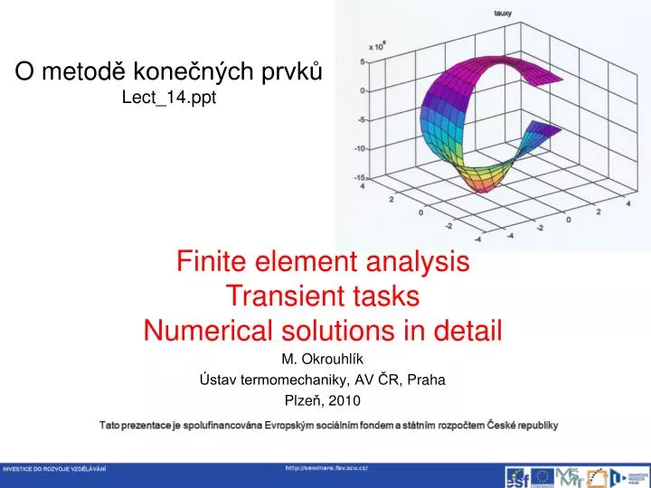
O metod ě konečných prvků Lect_ 14 .ppt. Finite element analysis Transient tasks Numerical solutions in detail. M. Okrouhlík Ústav termomechaniky, AV ČR , Praha Plze ň , 2010. www.it.cas.cz E:edu_mkp_liberec_2pdf_jpg_my_old_texts

E N D
O metodě konečných prvkůLect_14.ppt Finite element analysisTransient tasksNumerical solutions in detail M. Okrouhlík Ústav termomechaniky, AV ČR, Praha Plzeň, 2010
www.it.cas.cz E:\edu_mkp_liberec_2\pdf_jpg_my_old_texts\ Numerical_methods_in_computational_mechanics\Num_methods_in_CM.pdf
function [disn,veln,accn]=cedif(dis,diss,vel,acc,xm,xmt,xk,xc,p,h) % central difference method % dis,vel,acc ............... displacements, velocities, accelerations % at the begining of time step ... at time t % diss ...................... displacements at time t - h % disn,veln,accn ...........corresponding quantities at the end % of time step ... at tine t + h % xm ........................ mass matrix % xmt ....................... effective mass matrix % xk ........................ stiffness matrix % xc ........................ damping matrix % p ......................... loading vector at the end of time step % h ......................... time step % constants a0=1/(h*h); a1=1/(2*h); a2=2*a0; a3=1/a2; % effective loading vector r=p-(xk-a2*xm)*dis-(a0*xm-a1*xc)*diss; % solve system of equations for displacements using lu decomposition of xmt disn=xmt\r; % new velocities and accelerations accn=a0*(diss - 2*dis + disn); veln=a1*(-diss + disn); % end of cedif
SUBROUTINE CEDIF(XM,XM1,XK,DISS,DIS,DISN,VEL,ACC,P,R, 1 IMAX,NBAND,NDIM,H,EPS,IER,A0,A1,A2,A3,IMORE) C : : : : : : : DIMENSION XM(NDIM,NBAND),XM1(NDIM,NBAND),XK(NDIM,NBAND), 1 DISS(IMAX),DIS(IMAX),DISN(IMAX),VEL(IMAX),ACC(IMAX), 2 P(IMAX),R(IMAX) C C *** CASOVA INTEGRACE METODOU CENTRALNICH DIFERENCI *** C C SYSTEMU POHYBOVYCH ROVNIC TVARU C [M]{ACC}+[K]{DIS}={P} (TJ. SYSTEM BEZ TLUMENI) C SYMETRICKE PASOVE MATICE(MATICE HMOTNOSTI(POZITIVNE DEFINITNI), C REDUKOVANA EFEKTIVNI MATICE HMOTNOSTI,MATICE TUHOSTI) C JSOU usporne ULOZENY C V OBDELNIKOVYCH POLICH XM,XM1,XK O DIMENZICH NDIM*NBAND. C V PAMETI JE ULOZENA JEN HORNI POLOVINA PASU (VCETNE DIAG.). C C POZADOVANE PODPROGRAMY: C MAVBA ... NASOBENI SYMETRICKE PASOVE MATICE C VEKTOREM ZPRAVA C GRE ... RESENI SOUSTAVY LIN. ALGEBRAICKYCH ROVNIC C (GAUSSOVA ELIMINACE) C C PARAMETRY PROCEDURY: C C XM(NDIM,NBAND) ...... HORNI POLOVINA PASU MATICE HMOTNOSTI C XM1(NDIM,NBAND) ..... HORNI POLOVINA PASU REDUKOVANE C EFEKTIVNI MATICE HMOTNOSTI C XK(NDIM,NBAND) ...... HORNI POLOVINA PASU MATICE TUHOSTI C DISS(IMAX) .......... POSUVY V CASE T-H C DIS (IMAX) POSUVY V CASE T C DISN(IMAX) .......... POSUVY V CASE T+H C VEL(IMAX) ........... RYCHLOSTI V CASE T C ACC(IMAX) ........... ZRYCHLENI V CASE T C P(IMAX) ............. VEKTOR ZATEZUJICICH SIL (V CASE T) C R(IMAX) ............. VEKTOR EFEKTIVNICH ZATEZUJICICH SIL C IMAX ................ POCET NEZNAMYCH C NBAND ............... POLOVICNI SIRKA PASU (VCETNE DIAG.) C NDIM ................ RADKOVY ROZMER MATIC V HLAVNIM PROGRAMU C H ................... INTEGRACNI KROK C EPS ................. TOLERANCE (VIZ PROCEDURA GRE) C IER ................. CHYBOVY PARAMETR (VIZ PROCEDURA GRE) C A0,A1,A2,A3 ......... KONSTANTY METODY CENTRALNICH DIFERENCI C IMORE ............... = 0 POCITA POUZE POSUVY V CASE T+H C = JINA HODNOTA POCITA TAKE RYCHLOSTI C A ZRYCHLENI V CASE T+H C C ************************************************************** C C VEKTOR EFEKTIVNICH ZATEZUJICICH SIL V CASE T C {R}={P}-[K]{DIS}+A2*[M]{DIS}-A0*[M]{DISS} C CALL MAVBA(XK,DIS,VEL,IMAX,NDIM,NBAND) CALL MAVBA(XM,DIS,ACC,IMAX,NDIM,NBAND) CALL MAVBA(XM,DISS, R ,IMAX,NDIM,NBAND) C DO 10 I=1,IMAX 10 R(I)=P(I)-VEL(I)+A2*ACC(I)-A0*R(I) C C POSUVY V CASE T+H C CALL GRE(XM1,R,DISN,IMAX,NDIM,NBAND,DET,EPS,IER,2) C IF(IMORE .EQ. 0) GO TO 30 C C VYPOCTI TAKE RYCHLOSTI A ZRYCHLENI C DO 20 I=1,IMAX VEL(I)=A1*(-DISS(I)+DISN(I)) 20 ACC(I)=A0*(DISS(I)-2.*DIS(I)+DISN(I)) C 30 DO 40 I=1,IMAX DISS(I)=DIS(I) 40 DIS(I)=DISN(I) RETURN END
function [disn,veln,accn]=newmd(beta,gama,dis,vel,acc,xm,xd,xk,p,h) % Newmark integration method % % beta, gama ................ coefficients % dis,vel,acc ............... displacements, velocities, accelerations % at the begining of time step % disn,veln,accn ............ corresponding quantities at the end % of time step % xm,xd ..................... mass and damping matrices % xk ........................ effective rigidity matrix % p ......................... loading vector at the end of time step % h ......................... time step % % constants a1=1/(beta*h*h); a2=1/(beta*h); a3=1/(2*beta)-1; a4=(1-gama)*h; a5=gama*h; a1d=gama/(beta*h); a2d=gama/beta-1; a3d=0.5*h*(gama/beta-2); % effective loading vector r=p+xm*(a1*dis+a2*vel+a3*acc)+xd*(a1d*dis+a2d*vel+a3d*acc); % solve system of equations for displacements using lu decomposition of xk disn=xk\r; % new velocities and accelerations accn=a1*(disn-dis)-a2*vel-a3*acc; veln=vel+a4*acc+a5*accn; % end of newmd
A1=1./(BETA*H*H) A2=1./(BETA*H) A3=1./(BETA*2.)-1. A4=(1.-GAMA)*H A5=GAMA*H DO 10 I=1,NF DISS(I)=DIS(I) VELS(I)=VEL(I) 10 ACCS(I)=ACC(I) DO 40 I=1,NF 40 G(I)=A1*DISS(I)+A2*VELS(I)+A3*ACCS(I) C WRITE(1,900) A1,A2,A3,A4,A5 C900 FORMAT(" NEWM1 ",5G15.6) C WRITE(6,9010) BETA,GAMA,H,EPS,NF,NBAND,NDIM,IER C9010 FORMAT(" BETA,GAMA,H,EPS:",4G15.6/ C 1 " NF,NBAND,NDIM,IER:",4I6) C WRITE(1,901) G C901 FORMAT(" G PRED MAVBA"/(5G15.6)) CALL MAVBA(CMR,G,P,NF,NDIM,NBAND) C DO 45 I=1,NF C IF(P(I) .LT. 1.E-7) P(I)=0. C45 CONTINUE C WRITE(1,902) P C902 FORMAT(" P PO MAVBA"/(5G15.6)) DO 50 I=1,NF 50 G(I)=F(I)+P(I) C WRITE(1,903) G C903 FORMAT(" VEKTOR G PRED GRE"/(5G15.6)) C WRITE(6,919) C919 FORMAT(" CKR PRED GRE") C DO 920 I=1,NF C WRITE(6,904) I,(CKR(I,J),J=1,NBAND) C904 FORMAT(I6/(5G15.6)) C920 CONTINUE C IER=0 DET=0. CALL GRE(CKR,G,DIS,NF,NDIM,NBAND,DET,EPS,IER,2) C WRITE(6,906) DIS C906 FORMAT(" DIS PO GRE"/(5G15.6)) C DO 60 I=1,NF 60 ACC(I)=A1*(DIS(I)-DISS(I))-A2*VELS(I)-A3*ACCS(I) C DO 70 I=1,NF 70 VEL(I)=VELS(I)+A4*ACCS(I)+A5*ACC(I) RETURN END SUBROUTINE NEWM2(BETA,GAMA,DIS,VEL,ACC,F,NF,CKR,CMR,NDIM, 1 NBAND,H,EPS,IER,DISS,VELS,ACCS,P,G) C DIMENSION DIS(NF),VEL(NF),ACC(NF),F(NF),CKR(NDIM,NBAND), 1 CMR(NDIM,NBAND),DISS(NF),VELS(NF),ACCS(NF), 2 P(NF),G(NF) C C ***DIMENZIE VEKTOROV DISS,VELS,ACCS,G,P SA ROVNAJU*** C ***(2*POCTU UZLOV) DISKRETIZOVANEJ OBLASTI *** C C ***TATO PROCEDURA INTEGRUJE SUSTAVU POHYBOVYCH ROVNIC*** C ***NEWMARKOVOU METODOU S PARAMETRAMI BETA,GAMA *** C C ***VYZNAM PARAMETROV:*** C BETA,GAMA.......... PARAMETRE NEWMARKOVEJ METODY C DIS(NF) .......... NA VSTUPE-VEKTOR POSUVOV V CASE T C NA VYSTUPE-VEKTOR POSUVOV V CASE T+H C VEL(NF) .......... NA VSTUPE-VEKTOR RYCHLOSTI V CASE T C NA VYSTUPE-VEKTOR RYCHLOSTI V CASE T+H C ACC(NF) .......... NA VSTUPE-VEKTOR ZRYCHLENI V CASE T C NA VYSTUPE-VEKTOR ZRYCHLENI V CASE T+H C NF .......... POCET NEZNAMYCH JEDNEHO TYPU C CKR(NF,NBAND) ..... OBDELNIKOVA MATICE,OBSAHUJICI HORNI C TROJUHELNIKOVU CAST (VCETNE DIAGONALY) C EFEKTIVNI REDUKOVANE MATICE TUHOSTI. C T.J. [KRED]=[K]+A1*[M] PO PRUCHODU C GAUSSOVOU PROCEUROU GRE S KEY=1 C CMR(NF,NBAND) ..... OBDLZNIKOVA MATICA,KTORA OBSAHUJE HORNU C TROJUHOLNIKOVU CAST (VCITANE DIAGONALY) C SYMETRICKEJ,PASOVEJ,POZIT. DEFINITNEJ C MATICE HMOTNOSTI. C NBAND .......... POLOVICNA SIRKA PASU VCITANE DIAGONALY C NDIM .......... RIADKOVY ROZMER MATIC CKR,CMR,DEKLAROVANY C V HLAVNOM PROGRAME. C F(NF) .......... VEKTOR ZATAZENIA V CASE (T+H) C H .......... INTEGRACNY KROK C DISS(NF),VELS(NF),ACCS(NF) ..... HODNOTY Z PREDCHOZIHO KROKU C P(NF),G(NF) ....... PRACOVNI VEKTORY
Houbolt method FINITE ELEMENTPROCEDURES Klaus-Jürgen Bathe Professor of Mechanical Engineering Massachusetts Institute of Technology 1996 by Prentice-Hall, Inc. A Simon & Schuster Company Englewood Cliffs, New Jersey 07632 ISBN 0-13-301458-4
Houbolt procedure in Matlab function [disn,veln,accn] = ... houbolt(dis,vel,acc, diss,vels,accs, disss, velss, accss, xm,xd,xkh,p,h); % Houbolt integration method % disn, veln, accn new displacement, velocities, acceleration at t+h % dis, vel, acc displacement, velocities, acceleration at t % diss, vels, accs displacement, velocities, acceleration at t-h % disss, velss, accss displacement, velocities, acceleration at t-2*h % xm, xd mass and damping matrices % xkh Houbolt effective stiffness matrix % p loading vector at time t+h % h integration step % effective loading vector r=p+xm*(5*dis-4*diss+disss)/h^2+xd*(3*dis-1.5*diss+disss/3)/h; % new displacements disn = xkh\r; % new velocities and accelerations veln = (11*disn/6 - 3*dis + 3*diss/2 - disss/3)/h; accn = (2*disn - 5*dis + 4*diss - disss)/h^2; % end of houbolt
L1 element 1D continuum is a non-dispersive medium, it has infinite number of frequencies, phase velocity is constant regardless of frequency. Discretized model is dispersive, it has finite number of frequencies, velocity depends on frequency, spectrum is bounded, there are cut-offs. overestimated consistent Frequency (velocity) is with mass matrix. underestimateddiagonal
Dispersive properties of a uniform mesh (plane stress) assembled of equilateral elements, full integration consistent and diagonal mass matrices Direction of wave propagation Dispersion effects depend also on the direction of wave propagation Artificial (false) anisotropy How many elements to a wavelenght wavenumber
Correct determination of time step lmin … length of the smallest element c … speed of propagation tmin = lmin/c … time through the smallest element hmts … how many time steps to go through the smallest element h = tmin/hmts … suitable time step hmts < 1 … high frequency components are filtered out, implicit domain hmts = 1 … stability limit for explicit methods … 2/omegamax, where omegamax = max(eig(M,K)) hmts = 2 … my choice hmts > 2 … the high frequency components, which are wrong, due to time and space dispersion, are integrated ‘correctly’ LS Dyna uses h = 0.9*tmin as a default
Newmark vs. Houbolt _1 eps t = 1.6 dis 1.5 1.4 1.2 1 1 0.5 0.8 0 0.6 -0.5 0.4 0 0.5 1 0 0.5 1 vel acc 0 1.5 100 1 50 0.5 0 -50 -0.5 -100 0 0.5 1 0 0.5 1 L1 cons 100 elem Houbolt (red) Newmark (green), h= 0.005, gamma=0.5
Newmark vs. Houbolt _2 node = 101 L1 cons 100 elem Houbolt (red) Newmark (green), h= 0.005, gamma=0.5 1 0.03 0 0.02 -1 0.01 -2 0 -3 -0.01 0 100 200 300 400 0 100 200 300 400 history of strains (in time steps) history of displacement (in time steps) 1 100 0.5 50 0 0 -0.5 -50 -1 -100 0 100 200 300 400 0 100 200 300 400 history of velocity (in time steps) history of acceleration (in time steps)
A simple 1D study in Matlab To clarify the basic ideas of finite element (FE) computation, the relations between mechanical quantities and to show the behaviour of elastic stress waves in rods a simple FE program, utilizing 1D rod elements, was concieved. The program is based on assumptions of small displacement theory and linear elastic material response. J:\edu_mkp_liberec_2\tele_bk_2009_09_15_education_cd_jaderna_2005\11_computational aspects\A simple 1D study in Matlab_3.doc
Compare central differences vs. Newmark J:\edu_mkp_liberec_2\mtl_prog\matlab_prog_2010\mtlstep\barl1nc % barl1nc is a matlab program calculating the propagation of a strees % wave in a bar. The previous version is linbadh.m % Newmark and central difference methods are compared % strains, displacements, velocities and accelerations % along the bar are ploted for a given time % % time history of displacements, velocities and accelerations % of a chosen mode is recorded % % main variables % xm, xk, xd.............. global mass, rigidity and damping matrices % xme,xke ................ local mass and rigidity matrices % imax ................... number of generalized displacements % lmax ................... number of local degrees of freedom % kmax ................... number of elements % h ...................... step of integration % ityp ................... type of loading % = 1 .... Heaviside pulse % = 2 .... rectangular pulse % = 3 .... sine pulse % timp ................... length of pulse % delta .................. type of mass matrix % = 2/3 .... consistent % = 1 ...... diagonal % = 0.8 .... improved % gama ................... Newmark artificial damping parametr % tinc ................... time increment for plotting % tmax ................... maximum time % ck, cm ................. damping coeficients kmax=100 %input('number of elements=? (max 100) '); if kmax>200 , disp('linbad err. kmax>100'); break; end h=0.005; %input('integration step=? '); timp=0.25; %input('length of pulse=? '); delta= 1; %input('mass matrix'(2/3-cons) or (1-diag) or (0.8-improved)'); ityp=menu('Type of loading','heavi','rect','sin'); gama=0.5; %input('gama for Newmark '); ck=0; %input('damping coef. for rigidity matrix '); cm=0; %input('damping coef. for mass matrix '); tinc=0.1; %input('time increment for plotting '); tmax=0.5; %input('tmax=? '); Play with mass matrix formulation, time step number of elements conditional and unconditional stability numerical dumping
% barl1nhe % semantics: BAR - L1 1D elements - Newmark - Houbolt - Energy % % This is a matlab program calculating the propagation % of stress waves in a bar modelled by L1 elements % for three types of loading pulse. % Different types of right-hand side constraint are assumed. % Strains, displacements, velocities and accelerations % along the bar are ploted for a given time. % Strains, displacements, velocities and accelerations % for a given node are ploted as a function of time. % % Newmark and Houbolt methods are compared. % % Also potential kinetic and total energies are computed % at each time step and plotted at the end. % % main variables % xm, xk, xd.............. global mass, rigidity and damping matrices % xme,xke ................ local mass and rigidity matrices % imax ................... number of generalized displacements % lmax ................... number of local degrees of freedom % kmax ................... number of elements % h ...................... step of integration % ityp ................... type of loading % = 1 .... Heaviside pulse % = 2 .... rectangular pulse % = 3 .... sine pulse % timp ................... length of pulse % delta .................. type of mass matrix % = 2/3 .... consistent % = 1 ...... diagonal % = 0.8 .... improved % gama ................... Newmark artificial damping parametr % tinc ................... time increment for plotting % tmax ................... maximum time % ck, cm ................. damping coeficients Compare Houbolt vs. Newmark J:\edu_mkp_liberec_2\mtl_prog\matlab_prog_2010\mtlstep\barl1nhe4.m Play with mass matrix formulation, time step number of elements conditional and unconditional stability numerical dumping