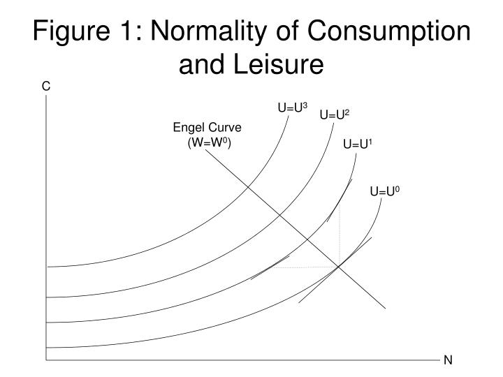
Figure 1: Normality of Consumption and Leisure

Figure 1: Normality of Consumption and Leisure C U=U3 U=U2 Engel Curve (W=W0) U=U1 U=U0 N

Figure 2: Long-Run Preferences and Technology Diagram (The Effect of an Increase in G) LMELR (W=W*) C MBLR (MBLR)´ C* C*´ N N* N*΄ -G -G’

Figure 3: A Higher W* Raises LMELR (the Engel Curve for W*) U=U3 (LMELR)´ (W=W*´) U=U2 U=U1 LMELR (W=W*) U=U0 N

Figure 4: Effect of an Increase in Z On Long-Run Equilibrium C (LMELR)´ LMELR (MBLR)´ MBLR C*´ C* N N*΄ N* -G

Figure 5: Illustration of Lemma 1 F ˆ F (ξ1,β,…) F (β,…) F (ξ0 ,β,…) F (ξ2,β,…) β

Figure 6:Felicity-Saving Possibility Frontier U slope= -Θ slope= -Θ ´ S

Figure 7: Money-Metric Net Felicity-Labor Possibility Frontier slope= -W slope= -W´ N

Figure 8: Effect of a Higher Wage on the U-S Possibility Frontier U N1 dW slope= -Θ slope= -Θ N2 dW S

Figure 9: The Effect of Higher N on Optimal C when UCN>0 UC ≈UCN(C,N) ΔN Θ UC(C,N2) UC(C,N1) C C2 C1

Figure 10: The Factor Price Possibility Frontier R slope= -N/K FPPF(Z) W

Figure 11: Labor Supply and Demand W Ns(Θ) + Nd(K,Z) + + N

Figure 12: Contemporaneous Preferences and Technology Diagram U=U0 C CMB [C=F(K,N,Z)-XK-G] N

Figure 13: The Investment Demand Curve θ λ ˆ II [θ=λ–q(X)] X

Figure 14: An Increase in Labor Supply W Ns(Θ) Ns(Θ´) Nd(K,Z) N

Figure 15: Consumption Falls When Θ Increases C W=W0 W=W1 N N0 N1

Figure 16: An Increase in K Raises Labor Demand W Ns(Θ) Nd(K΄,Z) Nd(K,Z) N

Figure 17: An Increase in K Causes a Movement Along the FPPF R K/N low K/N high FPPF(Z) W

Figure 18: An Improvement in Technology Shifts the FPPF Out R FPPF(Z) FPPF(Z΄) W

Figure 19: Comparative Statics of the Saving Supply Curve θ SS(k,Z,G) + + - X

Figure 20: The Effect of an Increase in X, Given K, Z and G U=U0 C U=U1 CMB0 C0 CMB1 [C=F(K,N,Z)-X1K-G] C1 N N0 N1

Figure 21: The Effect of an Increase in K, Given X, Z and G U=U0 C U=U1 CMB1 [C=F(K,N,Z)-XK1-G] C1 CMB0 C0 N N1 N0

Figure 22: Shifting Out the Investment Demand Curve (λ↑) θ SS λ1 θ1 λ0 θ0 ˆ II1 [θ=λ1-q(X)] ˆ II0 [θ=λ0-q(X)] X X1 X0

Figure 23: Shifting Out the Saving Supply Curve (K↑, Z↑, or G↓) θ SS0 SS1 λ θ0 θ1 ˆ II [θ=λ-q(X)] X X0 X1

Figure 24a: Phase Diagram with Upward-Sloping λ=0 Locus (Low Adjustment Costs) • λ • λ=0 saddle path • λ0 λ* • k=0 k k0 k*

Figure 24b: Phase Diagram with Vertical λ=0 Locus (Medium Adjustment Costs) • λ • λ=0 saddle path • λ0 λ* • k=0 k k0 k*

Figure 24c: Phase Diagram with Downward-Sloping λ=0 Locus (High Adjustment Costs) • λ • λ=0 saddle path • λ0 λ* • k=0 k k0 k*

Figure 25: II-SS When Moving Down the Saddle Path (K↑ and λ↓) θ SS(K0,Z,G) SS(K1,Z,G) λ0 θ0 λ1 θ1 ˆ II0 [θ=λ0-q(X)] ˆ II1 [θ=λ1-q(X)] X X1 X0

Figure 26a: DGE Effects of a Permanent Increase in G(Low Adjustment Costs) λ • λ=0 (old) • λ=0 (new) λ0 λ*new λ*old • k=0 (new) • k=0 (old) k k*old k*new

Figure 26b: DGE Effects of a Permanent Increase in G(High Adjustment Costs) λ • λ=0 (old) • λ=0 (new) λ0 λ*new λ*old • k=0 (new) • k=0 (old) k k*old k*new

Figure 27a: DGE Effects of a Permanent Increase in Z(Wealth Effect Dominates Rental Rate Effect) λ • • λ=0 (old) λ=0 (new) λ*old λ0 λ*new • k=0 (old) • k=0 (new) k k*old k*new

Figure 27b: DGE Effects of a Permanent Increase in Z(Rental Rate Effect Dominates Wealth Effect) λ • • λ=0 (old) λ=0 (new) λ0 λ*old λ*new • k=0 (old) • k=0 (new) k k*old k*new

Figure 27c: DGE Effects of a Permanent Increase in Z(Equal and Opposite Wealth and Rental Rate Effects) λ • • λ=0 (old) λ=0 (new) λ*old λ*new • k=0 (old) • k=0 (new) k k*old k*new

Figure 1: Normality of Consumption and Leisure