Download
1 / 12
120 likes | 290 Views
Numerical Cable Equalization. Hooman Hashemi 4/9/13. Cable Driving & Equalization. Good 2 rule of thumb: Linear increase of dB‘s with cable length Number of dB‘s increases with square root of F(MHz) Solutions we offer Use amplifiers to boost the higher frequency

E N D
Numerical Cable Equalization Hooman Hashemi 4/9/13
Cable Driving & Equalization • Good 2 rule of thumb: • Linear increase of dB‘s with cable length • Number of dB‘s increases with square root of F(MHz) • Solutions we offer • Use amplifiers to boost the higher frequency • Divide extreme equalizing designs into multiple “identical” cascaded stages • Excel sheet to compute the component values
Cable Driving & Equalization • Here you see a typical log log plot of cable loss vs. frequency • The Excel file provided uses this attenuation profile / expression (but it can be modified for a different cable) CAT5e (shielded twisted pair) 100ft response in log log plot
Component Design • Numerical Solution • Application note discusses this: Numerical Design • Uses Excel Solver function • It is modular- relatively easy to add more equalization banks • Component values can be changed “on the fly” with results immediately visible! • Uses Excel complex algebra capabilities to simplify computations Equalization Stage with 2 Banks 2-banks response on the left compared to 4-banks on the right
Component Design (Numerical Solution) • First need to compute the expression for gain • Can look difficult – at first • Can be simplified by considering equalization banks as “admittances” in parallel • Use Excel’s Complex arithmetic • Compute ” for each bank for all frequency of interest (in columns) and invert it to get the admittance of each bank • Sum all admittances, add to 1/RG, and invert to get ZG_eq • Having obtained ZG_eq, divide RF by it and add 1 to get “Vout/Vin” • Now you have the circuit’s gain expression plot • With more banks, copy and paste the cells to expand the spreadsheet →Equivalent Admittance = G1+G2+G3
Component Design (Numerical Solution) • Use “Complex” function to form the impedance made up of the resistance and the imaginary reactance • Use “IMDIV” to invert the bank impedances (ex: “IMDIV(1,D11)” ) before summing all the admittances with “IMSUM” to get the overall bank admittances • Add the overall bank admittances to 1/RG and invert in one shot to get ZG_eq • Continue using complex functions like “IMDIV”, “IMSUM”, and “IMABS” to get to the “1+RF/ZG_eq” which is the circuit gain expression • Superimpose plot of gain on cable attenuation to optimize design Cell H11 =IMSUM(IMDIV(1,D11),IMDIV(1,E11),IMDIV(1,F11)) Cell I11= IMDIV(1,IMSUM(1/RG,H11))
Component Design (Numerical Solution) • Limit each stage boost to 25dB or less • More than this may cause secondary effects, parasitic effects and other unexpected phenomenon to get in the way • Use “N” identical stages, each limited to 25dB max boost, cascaded • Design each stage boost for 1/N boost of the total boost needed (e.g. 50dB total boost with 2 stages would be 25dB / stage) • Use the Excel “Solve” function to minimize the difference between stage gain and cable attenuation with iteration • Define the Delta Function^2: (Difference between gain and cable attenuation)^2 • Select this as “Set Objective” and use “Min” • Specify the variables to change (in this case the R, and C values of the banks of one of the N stages) • Assign constraints • Click “Solve” • Start from low frequency and work your way upwards • May have to do this several times in succession • Verify your design using Spice • Build the amplifier and test with the cable Excel Solve window and its Settings 1-of-2-stages response on the left vs. 2-cascaded stages on the right
Component Design (Numerical Solution) • From Top LHS to Bottom RHS: • Used nominal starting values for R, and C (10k and 10pF) • Consecutive “Solve” iterations • Starting from low frequency and working upwards • May need to do several iterations • May decide to reduce # of banks if impact is low
Component Design (Numerical Solution) • These are the entries that need to be made in the Excel: • RF • RG • Bank values (R, and C) which is 4 in this case • N stages • Cable attenuation @ 10MHz for the length being used • Excel will compute the Gain and Cable attenuation plots and uses the following: • Delta^2= (Gain-Attenuation)^2 @ each frequency • Delta_Sum= Cumulative sum (from low to high frequency) of all “Delta^2” terms • This is the value which you use “Solve”, from low to high frequency, to optimize thereby driving down the total error between gain and attenuation • Bank values, and RG are the variables available for manipulation by “Solve • RF should be kept constant as it is usually not something with a lot of flexibility
Amplifier Choice • Desirable characteristics • Current feedback type (less effect on response with high frequency boost) • Here is the expression for current feedback closed loop gain: • “Rf+Ri(1+Rf/Rg)” can be defined as “Feedback Transimpedance” • Lower Ri (internal buffer output impedance) to lower unwanted response effects • Appropriate slew rate and large signal bandwidth for the signal amplitude and frequency • Capable to supporting the swing and output current needed
Simulation of Excel Results • The pole of these RC banks is the frequency beyond which the capacitor is considered a short and the bank impedance is equal to R • Looking at the poles for the Excel solution, the most likely pole would be the 1.7GHz one (R1, C1) • By reducing this pole, one has the highest chance of eliminating the phase margin issue that simulation has uncovered • The blog also investigates the design in TINA