Download
1 / 47
490 likes | 531 Views
Digital Image Processing. Intensity Transformations (Histogram Processing). Christophoros Nikou cnikou@cs.uoi.gr. Contents. Over the next few lectures we will look at image enhancement techniques working in the spatial domain: Histogram processing Spatial filtering

E N D
Digital Image Processing Intensity Transformations(Histogram Processing) ChristophorosNikou cnikou@cs.uoi.gr
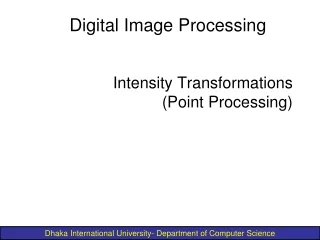
Contents Over the next few lectures we will look at image enhancement techniques working in the spatial domain: • Histogram processing • Spatial filtering • Neighbourhood operations
Image Histograms Frequencies Grey Levels The histogram of an image shows us the distribution of grey levels in the image Massively useful in image processing, especially in segmentation
Histogram Examples Images taken from Gonzalez & Woods, Digital Image Processing (2002)
Histogram Examples (cont…) Images taken from Gonzalez & Woods, Digital Image Processing (2002)
Histogram Examples (cont…) Images taken from Gonzalez & Woods, Digital Image Processing (2002)
Histogram Examples (cont…) Images taken from Gonzalez & Woods, Digital Image Processing (2002)
Histogram Examples (cont…) Images taken from Gonzalez & Woods, Digital Image Processing (2002)
Histogram Examples (cont…) Images taken from Gonzalez & Woods, Digital Image Processing (2002)
Histogram Examples (cont…) Images taken from Gonzalez & Woods, Digital Image Processing (2002)
Histogram Examples (cont…) Images taken from Gonzalez & Woods, Digital Image Processing (2002)
Histogram Examples (cont…) Images taken from Gonzalez & Woods, Digital Image Processing (2002)
Histogram Examples (cont…) Images taken from Gonzalez & Woods, Digital Image Processing (2002)
Histogram Examples (cont…) Images taken from Gonzalez & Woods, Digital Image Processing (2002) • A selection of images and their histograms • Notice the relationships between the images and their histograms • Note that the high contrast image has the most evenly spaced histogram
Contrast Stretching • We can fix images that have poor contrast by applying a pretty simple contrast specification • The interesting part is how do we decide on this transformation function?
Histogram Equalisation • Spreading out the frequencies in an image (or equalising the image) is a simple way to improve dark or washed out images. • At first, the continuous case will be studied: • r is the intensity of the image in [0, L-1]. • we focus on transformations s=T(r): • T(r) is strictly monotonically increasing. • T(r) must satisfy:
Histogram Equalisation (cont...) • The condition for T(r) to be monotonically increasing guarantees that ordering of the output intensity values will follow the ordering of the input intensity values (avoids reversal of intensities). • If T(r)is strictly monotonically increasing then the mapping from s back to r will be 1-1. • The second condition (T(r)in [0,1]) guarantees that the range of the output will be the same as the range of the input.
Histogram Equalisation (cont...) • We cannot perform inverse mapping (from s to r). • Inverse mapping is possible.
Histogram Equalisation (cont...) • We can view intensities r and s as random variables and their histograms as probability density functions (pdf) pr(r) and ps(s). • Fundamental result from probability theory: • If pr(r) and T(r) are known and T(r) is continuous and differentiable, then
Histogram Equalisation (cont...) • The pdf of the output is determined by the pdf of the input and the transformation. • This means that we can determine the histogram of the output image. • A transformation of particular importance in image processing is the cumulative distribution function (CDF) of a random variable:
Histogram Equalisation (cont...) • It satisfies the first condition as the area under the curve increases as r increases. • It satisfies the second condition as for r=L-1 we have s=L-1. • To find ps(s)we have to compute
Histogram Equalisation (cont...) Substituting this result: to yields Uniform pdf
Histogram Equalisation (cont...) The formula for histogram equalisation in the discrete case is given where • rk: input intensity • sk: processed intensity • nj: the frequency of intensity j • MN: the number of image pixels.
Histogram Equalisation (cont...)Example A 3-bit 64x64 image has the following intensities: Applying histogram equalization:
Histogram Equalisation (cont...)Example Rounding to the nearest integer:
Histogram Equalization (cont…)Example Images taken from Gonzalez & Woods, Digital Image Processing (2002) Notice that due to discretization, the resulting histogram will rarely be perfectly flat. However, it will be extended.
Equalisation Transformation Function Images taken from Gonzalez & Woods, Digital Image Processing (2002)
Equalisation Examples Images taken from Gonzalez & Woods, Digital Image Processing (2002) 1
Equalisation Transformation Functions Images taken from Gonzalez & Woods, Digital Image Processing (2002) The functions used to equalise the images in the previous example
Equalisation Examples Images taken from Gonzalez & Woods, Digital Image Processing (2002) 2
Equalisation Transformation Functions Images taken from Gonzalez & Woods, Digital Image Processing (2002) The functions used to equalise the images in the previous example
Equalisation Examples (cont…) Images taken from Gonzalez & Woods, Digital Image Processing (2002) 3 4
Equalisation Transformation Functions Images taken from Gonzalez & Woods, Digital Image Processing (2002) The functions used to equalise the images in the previous examples
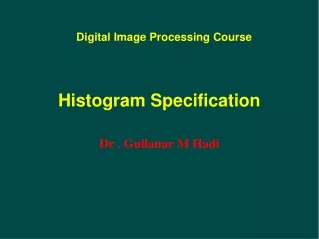
Histogram Specification Images taken from Gonzalez & Woods, Digital Image Processing (2002) • Histogram equalization does not always provide the desirable results. • Image of Phobos (Mars moon) and its histogram. • Many values near zero in the initial histogram
Histogram Specification (cont...) Images taken from Gonzalez & Woods, Digital Image Processing (2002) Histogram equalization
Histogram specification (cont.) Images taken from Gonzalez & Woods, Digital Image Processing (2002) • In these cases, it is more useful to specify the final histogram. • Problem statement: • Given pr(r) from the image and the target histogram pz(z), estimate the transformation z=T(r). • The solution exploits histogram equalization.
Histogram specification (cont…) Images taken from Gonzalez & Woods, Digital Image Processing (2002) • Equalize the initial histogram of the image: • Equalize the target histogram: • Obtain the inverse transform: In practice, for every value of r in the image: • get its equalized transformation s=T(r). • perform the inverse mapping z=G-1(s), where s=G(z) is the equalized target histogram.
Histogram specification (cont…) Images taken from Gonzalez & Woods, Digital Image Processing (2002) The discrete case: • Equalize the initial histogram of the image: • Equalize the target histogram: • Obtain the inverse transform:
Histogram Specification (cont...)Example Consider again the 3-bit 64x64 image: It is desired to transform this histogram to: with
Histogram Specification (cont...)Example The first step is to equalize the input (as before): The next step is to equalize the output: Notice that G(z) is not strictly monotonic. We must resolve this ambiguity by choosing, e.g. the smallest value for the inverse mapping.
Histogram Specification (cont...)Example Perform inverse mapping: find the smallest value of zq that is closest to sk: e.g. every pixel with value s0=1 in the histogram-equalized image would have a value of 3 (z3) in the histogram-specified image.
Histogram Specification (cont...)Example Images taken from Gonzalez & Woods, Digital Image Processing (2002) Notice that due to discretization, the resulting histogram will rarely be exactly the same as the desired histogram.
Histogram Specification (cont...) Images taken from Gonzalez & Woods, Digital Image Processing (2002) Original image Histogram equalization
Histogram Specification (cont...) Images taken from Gonzalez & Woods, Digital Image Processing (2002) Histogram equalization
Histogram Specification (cont...) Images taken from Gonzalez & Woods, Digital Image Processing (2002) Specified histogram Transformation function and its inverse Resulting histogram
Local Histogram Processing Images taken from Gonzalez & Woods, Digital Image Processing (2002) • Image in (a) is slightly noisy but the noise is imperceptible. • HE enhances the noise in smooth regions (b). • Local HE reveals structures having values close to the values of the squares and small sizes to influence HE (c).
Summary We have looked at: • Different kinds of image enhancement • Histograms • Histogram equalisation • Histogram specification Next time we will start to look at spatial filtering and neighbourhood operations