Download
1 / 46
460 likes | 489 Views
Metric Tensor: Application to Mesh Generation and Adaptation V. Selmin. Multidisciplinary Computation and Numerical Simulation. Unstructured Grid Generation. Advancing Front Method In the classical front advancing method, the nodes coordinates are built at the same time as the elements from

E N D
Metric Tensor: Application to Mesh Generation and Adaptation V. Selmin Multidisciplinary Computation and Numerical Simulation
Unstructured Grid Generation Advancing Front Method In the classical front advancing method, the nodes coordinates are built at the same time as the elements from the knowledge of the size of the elements that belong to the front and the spacing distribution. Delaunay Method In the Delaunay method, a triangulation of the domain from the knowledge of the boundary discretisation is first performed. Recursively, nodes are added in order to satisfy the imposed spacing distribution and new triangulation is performed in order to taking into account the insertion of new nodes. Metric Tensor and Mesh Spacing
Riemannian Metric A symmetric matrix A of range nxn is definite positive if The matrix A being symmetric, its eigenvalues are real and its n eigenvectors are orthogonal and form a basis. The vector q may be rewritten as a linear combination of the eigenvectors: where the are reals. That means that a definitive positive matrix have all its eigenvalues positive. Let a symmetric definitive positive tensor M(x) be defined at any point x of the computational domain . It represents a metric tensor if for any segment v the following relation holds: The tensor M(x) can be decomposed as Metric Tensor and Mesh Spacing
Riemannian Metric The matrix R is the orthogonal matrix of the normalised right eigenvectors of M(x) , computed at point x and is the diagonal matrix of eigenvalues. Moreover, is the orthogonal matrix of the normalised left eigenvectors. A transformation matrix T can be associated to M that is defined as By using the property of orthogonality ofv the eigenvectors of tensor M , we obtain and, consequently Metric Tensor and Mesh Spacing
: number of nodes in the element : coordinates of the nodes in space x : shape function in the space Optimal Elements A segment v contained in is optimal with respect to the given metric when it satisfied the relation An element is called optimal when its sides are optimal. Then the transformation T associated to M should transform an optimal element into an equilateral one with unitary side length. In the case of simplex elements (triangles and tetrahedra), there is only one value of M by which a given element is optimal. Let us indicate by the vector of lengths of the sides of the element, the components of the metric matrix M can be computed by solving the following linear system In the general case , the matrix M can be computed by taking advantage of the finite element theory. Let us indicate by the transformation that transforms an equilateral element in the parametric space into an element in the physical space x. Metric Tensor and Mesh Spacing
Optimal Elements The Jacobian of the transformation represents a transformation that accounts for the element size features in the physical space. In the finite element theory, the Jacobian is in general used to transform derivative operators from the physical to the parametric space whereas its transpose allows to compute spacing variations in the parametric space Therefore, the matrix may be defined as The determinant of the matrix is inversely proportional to the square of the element volume Metric Tensor and Mesh Spacing
Characteristic Dimension Parameters The geometrical characteristics of an element can be defined in terms of the following mesh parameters. If n is the number of dimensions, the parameters used are a set of n orthogonal directions and n associated element sizes . The transformation T may be defined as the result of superposing n scaling operations with factor in each direction: Therefore by taking into account that may be rewritten according to the following relations hold Metric Tensor and Mesh Spacing
Spacing in a given direction It can be desirable to limit the spacing in agiven direction. Let assume that a transformation T is defined at a given point x . At that point, we can associate to any direction, defined the versor , a scalar quantity, named spacing along the given direction, computed by using the following formula In order to impose the spacing l along a given direction , the transformation at the point has to be modified so that the new transformation matrix satisfies The transformation matrix is defined by the relation Metric Tensor and Mesh Spacing
Metrics Intersection The intersection of two transformation matrices and may be computed by using the following procedure. Let denote by the eigenvectors of one of the two transformation matrices – in general those that give the lowest spacing – and compute the element sizes according to The transformation matrix that results from the intersection of and may be written as This procedure allows to fully preserve the anisotropic character of the spacings, e.g. assuming that the element sizes defined by the two matrices are identical in one direction, but different along the others, the intersection matrix will maintain the spacing in those direction. Metric Tensor and Mesh Spacing
Mesh Spacing based on Interpolation Error Let be the Hessian matrix based on a quantity q and let assume that H(x) does not have zero eigenvalues. It can be decomposed as where R(x), L(x) are the Hessian normalised right and left eigenvectors matrices, respectively, and is the diagonal matrix of eigenvalues. The eigenvalues represent the second derivatives computed in a frame aligned with the Hessian eigenvectors. Let indicate by D(x) the matrix defined as The matrix D(x) is positive definite. It may be used to introduce a Riemann metric tensor defined by where k is a constant Metric Tensor and Mesh Spacing
Solution on the refined grid Solution on the initial grid Grid refinement Refined grid Initial Grid Sensor Build the metrics for the grid refinement and selection of the edges to be cut Metrics Refinement Concept Computation of the solution on the initial grid Sensor computation Grid refinement: Isotropic Anisotropic Build the refined grid and the interpolated solution Solution on the refined grid Mesh Refinement
T-1 Stretching direction Element to be refined Isotropic/Anisotopic Mesh Refinement Grid refinement strategy Hessian based Transformation Matrix Transformation matrix: Parameters: Mesh Refinement
Isotropic/Anisotopic Mesh Refinement Refinement criteria Triangular elements Quadrilateral elements Mesh Refinement
Isotropic/Anisotopic Mesh Refinement Grid refinement sensors • Type of sensors: • Based on • the quantity: q • the norm of gradient of the quantity: || q|| • the variation of the quantity along a specified direction: h q • n • Compressible Euler/Navier-Stokes equations: • Discontinuities such as shocks, contact discontinuities • Spurious total pressure loss • Shear layers (wakes, mixing layer, …) • Shock/boundary layer interaction zones • Refinement within the boundary layer sometimes not requested Mesh Refinement
Isotropic/Anisotopic Mesh Refinement Euler Grid: Anisotropic refinement, triangles RAE2822 Airfoil, M=0.75, α=3º Mesh Refinement
Isotropic/Anisotopic Mesh Refinement Euler Grid: Anisotropic refinement, quadrilaterals RAE2822 Airfoil, M=0.75, α=3º Mesh Refinement
Isotropic/Anisotopic Mesh Refinement Navier-Stokes Grid: Anisotropic refinement, quadrilaterals RAE2822 Airfoil, M=0.734, α=2.8º, Re=6500000 Mesh Refinement
cp t Mach Mach cp t Initial grid Refined grid Initial grid Refined grid Initial grid Refined grid Isotropic/Anisotopic Mesh Refinement Comparison between solutions computed on initial and refined grids Mesh Refinement
Quasi-structured reference grid: Init. Refin. Refer. NP 8360 8994 33440 NE 8200 8961 32800 NB 160 169 320 NI 164 164 328 Isotropic/Anisotopic Mesh Refinement Comparison between the solutions computed on the body with a reference solution Mesh Refinement
Node Movement Concept Linear spring analogy Spring Analogy: Source Term: Variational Analogy: Mesh Deformation
Node Movement Concept Basic Algorithm Spring Analogy: Algorithm: Differentiation: Mesh Deformation
Grid Deformation Aeroelastic Deformation Mesh Deformation
Grid Deformation Movement of Wing/Pylon/Nacelle/Sponson System on the Fuselage Mesh Deformation
Grid Deformation Movement of Wing/Pylon/Nacelle/Sponson System on the Fuselage Mesh Deformation
Adaptation through Grid Deformation Euler Grid: Adaptation through node movement, triangles NACA0012 Airfoil, M=0.85, α=1º Mesh Deformation
Adaptation through Grid Deformation Euler Grid: Adaptation through node movement, quadrilaterals NACA0012 Airfoil, M=0.85, α=1º Mesh Deformation
Mesh Generation-Unstructured Grids Unstructured Advancing front method (Tetrahedra) III phases: 1 - Discretisation of the curves (points) 2 - Discretisation of the surfaces (triangles) 3 - Discretisation of the volume (tetrahedra) Need a system which provides the spacings within the whole computational domain Use the concept of Riemannian metrics in order to work in the normalised space. High flexibility for the discretisation of complex geometries Mesh Generation
Mesh Generation-Unstructured Grids Old system to provide the spacings based on elementary solids (spheres, cylinders, troncated cones, …) Mesh Generation
Mesh Generation-Unstructured Grids New mesh generation procedure requirements 1- Anisotropic Mesh Generation Needed for boundary layer discretisation (hybrid grids) and control of the number of nodes (stretching along wing span) 2- High Flexibility in Mesh Generation For surface grid and volumic grid generations 3- Automatic Background Grid Computation From metrics on the surface to metrics in the volume 4- Grid Quality Fast grid generation is important but high quality grid is far more important - A posteriori grid quality improvement tool Mesh Generation
Mesh Generation-Unstructured Grids From metrics on the surface to metrics in the volume 1- Compute the associated mesh metrics starting from the discretisation of the body skin & the external boundary 2- Form the node connectivity by using Delaunay algorithm 3- Build additional nodes and formed links to nodes on the body 4- Compute metrics for the additional nodes 5- Eventually, correct the computed metrics 6- Connect all the nodes by using Delaunay algorithm 7- Metrics in any point by interpolation on the last Delaunay grid Mesh Generation
Mesh Generation-Unstructured Grids Metrics on the surface 1- Computation of the principal curvatures and principal curvature directions on the surface by using the mathematic definition of the surfaces. 2- The principal curvature directions are orthogonal and will defines the spacing directions in plane tangent to the surface at a given points. 3- The spacing along the principal curvature directions will be computed as a fraction of the curvature radius associated to the principal curvatures 4- The spacing has to be limited by threshold values (maximum and minimum spacing allowed), in order to control the spacing . This is particular true when the curvature radius is very large (case of planes). 5- The third direction is computed as the vectorial product of the first two. The spacing in this direction is computed as the minimum of the first two spacings. 6- In general, discontinuities in metrics are present from a surface to its adjacent surfaces. A smoothing procedure is applied in order to regularise the metrics. Mesh Generation
Mesh Generation-Unstructured Grids Elementary Differential Geometry of Surfaces Equation of surface: Normal vector to the surface Equation of a curve on the surface Unit tangent vector along a curve Mesh Generation
Mesh Generation-Unstructured Grids Normal curvature to a surface: Principal direction of normal curvature Principal curvatures Gaussian curvature Mean curvature Mesh Generation
Mesh Generation-Unstructured Grids Mesh spacing based on local curvature Mesh spacing along curve: Mesh spacing along principal curvature directions Correction of mesh spacing Metric tensor Mesh Generation
Grid: 12000 nodes on skin, 210000 nodes in total Grid: 15000 nodes on skin, 284000 nodes in total Mesh Generation-Unstructured Grids Mesh Generation
Mesh Generation-Unstructured Grids Mesh Generation
Mesh Generation-Unstructured Grids Mesh Generation
Mesh Generation-Unstructured Grids Mesh Generation
Mesh Generation-Unstructured Grids Mesh Generation
Mesh Generation-Unstructured Grids Mesh Generation
Mesh Generation-Hybrid Grids Hybrid Grids Mesh Generation (Prisms+Tetrahedra) – Strong formulation II phases: 1- Build the pseudo structured layers from the discretised surface 2- From the outer layer build the grid formed by tetrahedra Mesh Generation
Mesh Generation-Hybrid Grids Application to Hybrid Grid Generation (2D & 3D) Mesh Deformationt
Mesh Generation-Hybrid Grids Hybrid Grids Mesh Generation (Prisms+Tetrahedra) – Weak formulation II phases: 1- Build the tetrahedra based unstructured grid. 2- For each layer that will be added, compute the normal vector and the displacement values 3- Compute the force, that should give the required displacement effect (source term). 4- Applied the node movement procedure. NB: The layer at the beginning of the node movement process has a zero thickness. In general, the weak formulation allows to better control possible layers overlapping near concave regions. It results also in smoother grids. Mesh Deformationt
Skin Outer boundary layer Mesh Generation-Hybrid Grids 560000 nodes, 30 layers in the B.L. region. Mesh Deformationt
Mesh Generation-Hybrid Grids 560000 nodes, 30 layers in the B.L. region. Mesh Deformationt
Summary Riemannian metrics Spacing distribution and stretching Mesh Refinement Isotropic Mesh Refinement Anisotropic Mesh Refinement Node Movement Grid deformation (aeroelasticity, optimisation, …) Grid adaptation Mesh Generation (viscous layers) Advanced Mesh Generation Spacing on surfaces driven by curvature Background spacing on the surface for control purpose Automatic system to build mesh spacing in the volume Anisotropic spacing Hybrid grid generation Mesh Deformationt