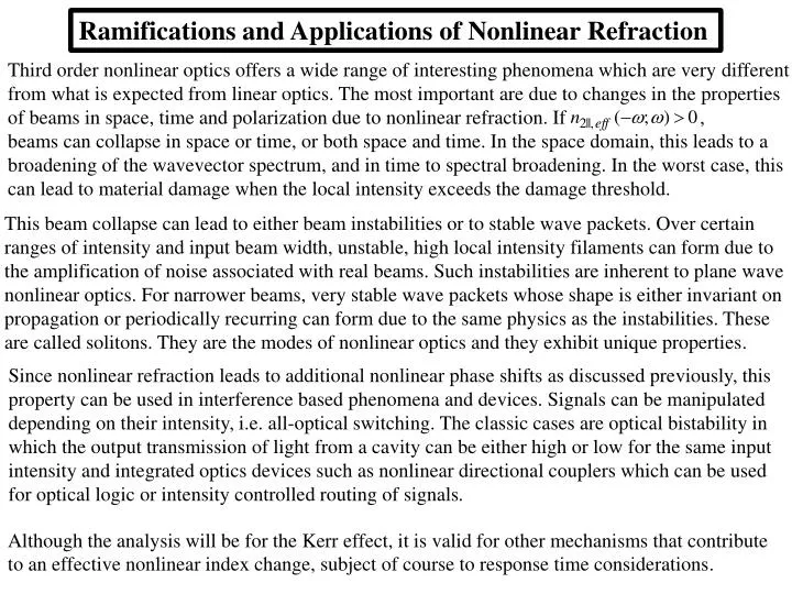
Ramifications and Applications of Nonlinear Refraction

1. Ramifications and Applications of Nonlinear Refraction Third order nonlinear optics offers a wide range of interesting phenomena which are very different from what is expected from linear optics. The most important are due to changes in the properties of beams in space, time and polarization due to nonlinear refraction. If , beams can collapse in space or time, or both space and time. In the space domain, this leads to a broadening of the wavevector spectrum, and in time to spectral broadening. In the worst case, this can lead to material damage when the local intensity exceeds the damage threshold. This beam collapse can lead to either beam instabilities or to stable wave packets. Over certain ranges of intensity and input beam width, unstable, high local intensity filaments can form due to the amplification of noise associated with real beams. Such instabilities are inherent to plane wave nonlinear optics. For narrower beams, very stable wave packets whose shape is either invariant on propagation or periodically recurring can form due to the same physics as the instabilities. These are called solitons. They are the modes of nonlinear optics and they exhibit unique properties. Since nonlinear refraction leads to additional nonlinear phase shifts as discussed previously, this property can be used in interference based phenomena and devices. Signals can be manipulated depending on their intensity, i.e. all-optical switching. The classic cases are optical bistability in which the output transmission of light from a cavity can be either high or low for the same input intensity and integrated optics devices such as nonlinear directional couplers which can be used for optical logic or intensity controlled routing of signals. Although the analysis will be for the Kerr effect, it is valid for other mechanisms that contribute to an effective nonlinear index change, subject of course to response time considerations.

2. Vp' Self-focusing Local phase velocity Vp' Self-defocusing Vp > Vp' Self-focusing and Defocusing of Beams This phenomenon is associated with beams of finite cross-section. An intensity dependent change in the refractive index or a cumulative nonlinear phase shift can be created by a beam. Hence the beam introduces an effective lens in the medium which affects the propagation of the beam itself, and any other beam present. • - The larger the refractive index n, the slower the phase velocity • For , high intensity region travels slower than wings → curvature of phase front. For , self-defocusing occurs and beams spreads, augmenting diffraction. Vp > Vp'

3. “External Self-action” (thin sample) The shape of the beam is not significantly changed inside the sample and only the beam’s phase front is augmented by on transmission. Assuming a lossless gaussianbeam and no diffraction inside the sample, i.e. z0>>L, For small phase distortion, the exponential can be expanded as where numerical simulations have shown that C3.77 is a good approximation. Compare to action of lens of focal length “f” in linear optics, “External Self-action” (thick sample) In this case the beam profile collapses for inside the nonlinear medium. There is a critical power Pc (or intensity Ic) for collapse.Assume diffraction occurs over the characteristic distance for which and ,

4. in which zf is the distance to the “focus”.Typical numbers for critical power are: CS2,  4.5x10-14cm2/W and n1.6 at vac =1mPc  30KW; fused silica,  2.5x10-16cm2/W and n1.5 at vac1m  Pc 3.5MW. In practice, catastrophic self-focusing is arrested by other physical nonlinear effects such as ionization, stimulated scattering, multi-photon absorption, electron plasma formation etc. Furthermore, the scalar and paraxial models break down when w0→and the term ignored in the paraxial approximation must be included. The term also mixes all three field components so that for a polarized input, radiation rings of both transverse polarizations are emitted. Periodically foci occur with distance, the higher the input intensity, the more frequent the focal spots. The picture illustrates what occurs in air. The preceding discussion was based on Kerr nonlinearities. The same self-focusing phenomenon occurs under appropriate conditions for all third order nonlinearities. However, the governing equations can be more complex and need to be tailored to the individual nonlinear mechanisms. Non-locality involving diffusion of the index change in space as found in liquid crystals, photorefractive media, thermal effects, charge carrier nonlinearities in semiconductors, etc. tend to counter-act self-focusing and raise the power required for self-focusing. Self-focusing also occurs for the “cascading” nonlinearity.

5. “Self-phase Modulation” and Spectral Broadening in Time Just as in the space domain, pulse broadening occurs for and pulse narrowing for . In the absence of nonlinearity, pulse broadening always occurs due to Group Velocity Dispersion (GVD) which is the equivalent of diffraction in the space domain. Note that the sign of NL changes from the leading (T<0) to the trailing edge (T>0) of the pulse.The spectral broadening can be quite large. For example in fibers, is feasible.Such large spectral broadening is easily measurable with a spectrum analyzer. The frequency spectrum is , i.e. There are points on the pulse envelope for which the frequencies are equal leading to interference in the spectral domain. As a result the spectrum is periodic in

6. Beam Instabilities in Space Plane waves are the normal modes of linear optics, but as will be shown here they are subject to instabilities under the appropriate conditions on intensity in nonlinear optics. The results derived here are valid for plane waves or very wide (relative to a wavelength) beams. Recall from the discussion on nonlinear diffraction There is always “noise” on any real beam which can be Fourier analyzed to give a noise magnitude at the spatial frequency κ. Therefore a real beam with nonlinearity present can be written as A real indicates that the noise grows exponentially with distance in the small signal gain approximation and, since the noise is amplified, the plane wave solution is unstable. The solution field and are introduced into the nonlinear wave equation which includes diffraction A solution exists only for a self-focusing nonlinearity, and for

7. The noise with spatial κis amplified once the intensity crosses a threshold value which is different for every value of κ. Note that the larger the periodicity , the lower the threshold for instability. I1>I2 The analysis has been given for a plane wave. However, MI also occurs for wide beams as long as their half-width is much greater than the MI period associated with their peak intensity. An experimental example is shown for slab AlGaAs waveguides ( ) which are effectively a 1D system since diffraction can occur only in the plane of the waveguide. Input beam Although the analysis above has been for Kerr nonlinearities, MI is a universal phenomenon in nonlinear optics and occurs for all self-focusing nonlinearities.

8. Instabilities in Time The temporal case is a complete analogue to the spatial case, with GVD replacing diffraction. GVD and Pulse Broadening In the frequency domain, the linear wave equation for a pulse with central frequency a is Expanding , again for pulses many cycles long GVD Fourier transform into time domain and transforming to co-ordinates travelling with pulse (T).

9. e.g. Ldisis the characteristic dispersion length for pulse broadening. Note the sign of the frequency shift across the pulse for k2<0is opposite to that for self-phase modulation. Also, the pulse width increases on propagation for both signs of k2. Pulsed and cw beams can also have instabilities in the time domain. Repeating the previous space domain analysis modified for the time domain Fused silica glass In contrast to spatial diffraction which has only one sign, both signs for GVD exist. For example, in fused silica the sign changes from positive to negative at 1.3m. MI can only occur for fused silica which has for wavelengths longer than 1.3m .

10. Solitons(Nonlinear Modes) Soliton are robust solutions to the nonlinear wave equations that correspond to beams which do not spread or collapse in space or time, or both under appropriate conditions. In the linear optics case, solutions to Maxwell’s equations are eigenmodes, i.e. they satisfy orthogonality conditions. This is not the case for solitonsalthough by satisfying the nonlinear wave equation they are modes. Solitons have some very special (unexpected from linear optics) properties. Bright solitons exist in all media which exhibit self-focusing. There are also solitonsin self-defocusing media, called dark or grey solitons. Mathematically they consist of a notch in a plane wave. In practice the wider the extent of the field in which the notch exists, the more stable is the dark soliton.The only nonlinearity for which realistic analytical solutions exist is the Kerr case. (Other cases need to be analyzed numerically.) The simplest (and only stable) Kerr case is for a single dimension in which light can spread in space or time, spatial solitons and temporal solitons respectively. Bright Kerr Solitons These solitons are only stable in 1D. Spatial Solitons Light is guided by a thin film of higher refractive index than the surrounding media. The fields decay evanescently into the surrounding media. Hence diffraction can only occur in the plane of the film. The guided wave field polarized in the plane of the surfaces has the form

11. There exists a simple criterion for the existence of 1D spatial solitonsof arbitrary order in terms of diffraction length and the nonlinear length , namely LDif=N2LNL with N=1. There exist higher order spatial (and temporal) solitons with the order given by N=2, 3.. which have progressively higher power requirements. There is periodic evolution of the N>1 solitonfields with distance. The period is In addition to the properties already discussed, solitons have other “unusual” properties. Solitonsare robust against fluctuations in width or power, i.e. aPsol = constant for 1D Kerr media. Since dPsol/da< 0, Psola-1 and vice-versa, any increase in the soliton power is compensated for by a decrease in the width. This also holds for non-Kerr solitons. i.e. any decrease in Psol is still compensated by an increase in width and vice-versa. 2. Solitons have fascinating collision properties. They act like both waves and particles. In the Kerr case, the number of output solitons=the number of input solitons. Nevertheless, in the overlap region, obvious interference effects occur. There are attractive and repulsive forces which depend on the relative phase angle between interacting solitons.

12. Δ=/2 Δ=0 Δ= Δ=0 3. Kerr solitons are impervious to small perturbations, i.e. they are not scattered by them. 4. Solitons, with the exception of those due to cascading, can form waveguides which can trap other weaker beams at a different frequency or polarization or both. Temporal Solitons The analysis of this case and hence many of the unique features of temporal solitonsare analogous to the spatial case which has been discussed in some detail already. The soliton field is Some typical numbers for silica fibers at =1.55mare k2=-20ps2/km, Psol=5W for T0=1ps, and Psol=50mW for T0=10ps. The original proposal for communications was to use 10ps pulses. A property not yet discussed is the excitation of solitons with inputs of the wrong shape and peak power. Shown is the evoluton into a soliton of a Gaussian input beam with N=0.75. This is a direct consequence of the soliton robustness property.

13. Dark Kerr Solitons Temporal dark solitonsexist for and . The starting nonlinear wave equations are the same as for bright solitons, but the solutions for are of course different. Note that the dark soliton is a “notch” in an infinite broad plane wave background and hence requires, in principle, infinite energy. There is a π phase difference between the background fields on opposite sides of the notch. If this phase difference is less than π, the notch does not go tozero (grey soliton) and the notch has a “transverse velocity”, i.e. it travels at an angle (slides sideways along the time axis). It is clearly not possible to satisfy the theoretical conditions of an infinitely broad background. However, since solitons are robust, solitoniceffects are visible for finite width beams and short propagation distances. Dark temporal solitons require the product so in principle can occur for the combinations as well as . However, since diffraction has only one possible sign, namely negative, dark spatial solitons require a defocusing nonlinearity.

14. Bright Solitonsin Space and Time (Optical bullets) The condition for solitons in both space and time can be written as y Normal pulses “Light bullet” t To date it has not proven possible to get light bullets in 2D. A light bullet in quasi-1D for which one dimension is large and the spreading of the second (narrow) dimension is compensated by nonlinearity was demonstrated using the cascading nonlinearity. Experimental Results

15. Optical Bistability For an input into an appropriate “cavity”, for example a Fabry-Perot interferometer, and under certain conditions of initial detuning of the cavity from one of its transmission resonances, the output has two possible states of cavity transmission for a range of input powers. The actual output state obtained depends on whether the input was decreasing or increasing in power when approaching these states, i.e. the previous history of the input beam. R and T, areintensity reflection and transmission coefficients Unidirectional Cavity Total round trip phase shift is

16. This behavior can be explained as follows. Starting on resonance, increasing the input intensity results in a nonlinear phase shift which tunes the total phase off the resonance peak so that the transmission decreases and the output intensity becomes sub-linear in the input intensity, case (b). For initially negative detuning, the transmission increases with input intensity as the system moves towards the resonance due to the nonlinear phase shift, i.e. the output increases faster than linear in the input, case (c). In this region, . When resonance is reached, further increases in input intensity move the system off resonance and the response is similar to case (b). In case (d), a “run-away” effect takes place in which an increase in input intensity moves the system further towards the resonance and reaches a point where the increase in the cavity field and hence the nonlinear phase shift is large enough to continuously move the system to resonance without further increase in the input intensity. This corresponds to a region (dashed black line) where stability analysis shows the system is unstable. The system “jumps” to the high transmission state. Subsequent increase in input intensity produces behavior similar to (b). When decreasing the input intensity from above the hysteresis loop, the cavity field starts in the high transmission state. The cavity field decreases but remains in the high transmission state until the system becomes unstable and can no longer stay on resonance at which point it jumps” down to the low transmission state. Hence a hysteresis loop is formed due to the feedback provided by the cavity! Which state the system is in depends on the prior history of the illumination.

17. All-optical Signal Processing and Switching Because of the importance of controlled routing of optical signals in communications, a number of schemes have been developed for using light to control light which in principle can be achieved in shorter times than by electronics which is limited by electron transit times across some junction. This can be implemented by using the intensity-dependent refractive index in control-signal beam geometries using waveguides in either fiber or channel integrated optics form. Linear Coupler A linear directional coupler consists of two parallel identical channel waveguides in which the optical field in one waveguide overlap the second waveguide. When one waveguide is excited, light transfers with propagation distance to the second waveguide. The distance required for complete transfer is called the coupling length LC. Two simple coupled wave equations describe the response of the system, namely If the two waveguides are slightly mismatched with propagation constants , i.e. with a characteristic beat length , the coupled wave equations become

18. Clearly mismatching the waveguides reduces the coupling significantly. This can be quantified by R=2LC/Lb. Nonlinear Directional Coupler If the coupler is made of a nonlinear material with the coupler can be mismatched by increasing the intensity. For , the coupled equations become Solid red – R=0. Dashed red – R=1. Solid blue – R=2. Dashed blue – R=8. The nonlinearity is given in terms of  by Analytic solutions are given by Jacobi elliptic functions in terms of a critical power .

19. Red curves: dashed P1(0)/Pc=0.4, solid P1(0)/Pc=0.95. Black curve: P1(0)/Pc=1.0. Blue curve: dashed P1(0)/Pc=2, solid P1(0)/Pc=1.05. (b) Red curve: P1(0)/Pc=0.9999. Black curve: P1(0)/Pc=1.0. Blue curve: P1(0)/Pc=1.0001. Exactlyat P1(0)=Pcin the asymptotic limit of a very long coupler, L>>LC) the power is split 50:50 between the waveguides. This an unstable point and the slightest deviation upwards in power leads to oscillations Far above the critical power, there is essentially no power transfer to waveguide 2. Therefore, in going from low to high power, the signal is switched between channels. The behavior of this device is also non-reciprocal for initially detuned devices. If and with power incident in channel 1, the power-dependent increase in initially increases the power transfer to channel 2 where-as if , inhibits the transfer of power to channel 2.

20. A potential application of this device to demultiplexing or routing. The strong control pulse (red) in the lower channel detunes the coupler during its passage through the device. No signal can cross out of the signal channel if it is coincident with the control pulse. The control pulse can be orthogonally polarized, or even be at a different frequency.