Observational data-driven surface concentration derived from satellite columns

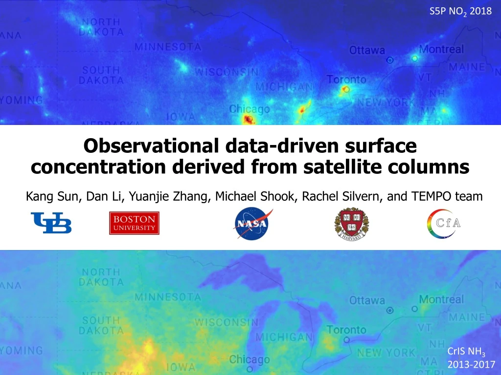
1. S5P NO2 2018 Observational data-driven surface concentration derived from satellite columns Kang Sun, Dan Li, Yuanjie Zhang, Michael Shook, Rachel Silvern, and TEMPO team CrIS NH3 2013-2017

2. Introduction • Satellite data provide excellent spatiotemporal coverage • Emissions, distributions, trends of pollutants (NO2, HCHO, NH3, SO2 …) • However, satellite products are often vertical (sub) column density, instead of surface concentrations • Regulations, exposure, land-atmospheric exchange, intercomparisons • Profiles simulated by a chemical transport model (CTM) are conventionally used to infer surface concentrations from satellite columns CrIS NH3 Kharol et al. 2018 OMI-GEOS-Chem NO2 Lamsal et al. 2013 OMI-GEOS-Chem HCHO Zhu et al. 2017

3. PBLH in CTMs • It is a challenge to accurately model boundary layer processes in meteorological models and CTMs • GEOS-Chem is driven by GEOS-FP or MERRA-2 • CMAQ/WRF-Chem are often driven by NARR • Computationally demanding to match CTM with the spatiotemporal coverage and spatial resolution of next generation satellites GEOS-FP PBLH vs. high spectral resolution lidar (HSRL) PBLH (Zhu et al. 2016) NARR PBLH vs. CALIPSO PBLH (2012-2013) CALIPSO data from Ralph Kuehn, SSEC UW-Madison

4. Column to surface volume mixing ratio (VMR) • Vertical column Ω integrated from surface pressure ps to upper boundary pt; q is specific humidity; g is gravitational acceleration; MA is dry air molecular mass; x(p) is VMR profile: • Define shape factor γ as (PBLP is thickness of PBL in pressure): • Apparently γ = 1 if • Combining (1) and (2): (1) (2)

5. Representing profiles • g and MA are constants • Ω is readily available from satellite products, with error estimation and validation • γ represents how the profile distributes in and out of the PBL • PBLP is closely related to the physical height of PBL (PBLH) • Is it possible to obtain the profile distribution and PBL thickness from observations? • Hypothesis 1: the profile shapes for reactive species (NO2, HCHO, NH3) have some level of similarity and γdoes not need to be spatiotemporally resolved • Hypothesis 2: PBLH/P can be unbiasedly determined by combining observations and reanalysis

6. Determining γ by dimensional analysis • The lifetimes of target species (e.g., NO2, HCHO) are longer than PBL mixing time scale (< 1 hour), but shorter than the exchange time scale between PBL and free troposphere (~ 1 day) • The sources and sinks are mainly in the PBL • Five relevant variables: p, ps, PBLP, x, xPBL (average PBL concentration) • Three primary dimensions: length, mass, time • Buckingham-PI (∏) theorem: 5-3 = 2 dimensionless groups • As a dimensional analysis exercise, the functional relationship f() has to be determined from observations • γis readily determined from f()

7. NASA DISCOVER-AQ campaigns Systematic sampling of PBL/lower FT 838 spirals ~5 km diameter With missed approaches down to ~30 m AGL 4-17 local sun time

8. Determining PBLP/H from DAQ profiles • Top of PBL manually labelled from DISCOVER-AQ profiles (MD: 253, CA: 170, TX: 195, CO: 220) based on multiple tracers • Compared with independent manual labels for MD (Don Lenschow) and CA (Michael Shook)

9. Similarity in dimensionless profiles: NO2 Grouped by campaigns, 12-14 local time Grouped by local time, all campaigns

10. Similarity in dimensionless profiles: HCHO Grouped by campaigns, 12-14 local time Grouped by local time, all campaigns

11. Observational data-driven PBL thickness • Meteorological data records when commercial aircrafts take off/land • Aircraft Meteorological Data Reports orAMDAR • UScontributionsarealsooftencalledACARS • PBL profiles at hourly scales based on AMDAR/ACARS Zhang et al. JGR 2018 ACARS PBLH

12. Validating ACARS PBLH • ACARS: • Continuous, hourly observations • Low bias • Sparse in space • Reanalysis (e.g., NARR) • Spatial/temporally resolved • Comprehensive geophysical variables (T, wind, fluxes) • Variant biases • Data-driven model to merge both datasets • Collaboration with Dan Li, Boston University MD: BWI, PHL, DCA TX: IAH, HOU CO: DEN

13. Physical oversampling surface concentrations • x(i): derived surface VMR at pixel i; x(j): mean value at grid j • S(i,j) is the integrated spatial sensitivity of satellite pixel i over the area of grid cell j • σ(i) is the error of derived surface VMR, estimated by error propagation: Sun, Zhu et al. AMT 2018

14. Application for TEMPO • Ensemble average of dimensionless aircraft profiles approximate profiles seen by a TEMPO pixel • Diurnal profile shape evolution in DISCOVER-AQ data can be leveraged for TEMPO • Commercial airline data (ACARS) capture diurnal variation of PBLH • Besides NARR, HRRR PBLH are available at 3-km, 1-hour resolutions over CONUS from 2016

15. Free trop background?

16. DISCOVER-AQ spiral PBLH overview

17. Profile shapes in CTMs: comparison • Observed profiles: DISCOVER-AQ MD (top) and CA (bottom) • Filtered by 10-15 local time • CTM: nested GEOS-Chem0.5°×0.625° horizontal resolution over North America • Driven by MERRA-2 • Sampled at spiral locations and 13:30 local time • CTM shows lower gradients at PBL/lower troposphere • Computationally demanding to match CTM with the spatiotemporal coverage and spatial resolution of next generation satellites Observation-based profiles (γ and PBLP)?

18. Similarity in dimensionless profiles: NH3 Grouped by campaigns, 12-14 local time Grouped by local time, all campaigns