 z , I

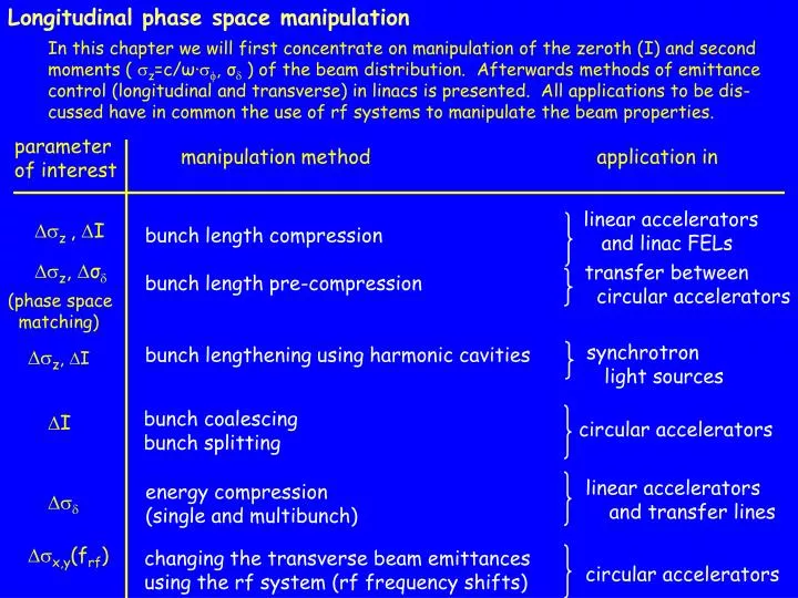
1. Longitudinal phase space manipulation In this chapter we will first concentrate on manipulation of the zeroth (I) and second moments ( z=c/ω·, σ ) of the beam distribution. Afterwards methods of emittance control (longitudinal and transverse) in linacs is presented. All applications to be dis- cussed have in common the use of rf systems to manipulate the beam properties. parameter of interest manipulation method application in linear accelerators and linac FELs z , I bunch length compression bunch length pre-compression bunch lengthening using harmonic cavities z, σ transfer between circular accelerators (phase space matching) synchrotron light sources z, I bunch coalescing bunch splitting I circular accelerators linear accelerators and transfer lines energy compression (single and multibunch)  x,y(frf) changing the transverse beam emittances using the rf system (rf frequency shifts) circular accelerators

2. Introduction e+/-: =momentum compaction factor p: -1/γt2 2πfrf single-particle equation of motion energy deviation E=beam energy T=revolution period phase deviation derivatives wrt time, t  harmonic oscillator equations (=s,=0) =t ellipses in phase space (for linear rf; i.e. small amplitude particle motion) synchrotron frequency synchrotron tune

3. Analogy between transverse and longitudinal motion transverse longitudinal kx .. px + kpx = 0 equations of motion k  (/c)^2 x’  (xco+x=0, x’co+x’=0) (=s,=0) x =t phase space second moments beam matrix (taking <x>=0, <x’>=0) (taking <>=0, <>=0) emittance

4. Bunch length compression motivation: produce short bunches (at expense of increased energy spread) in order to minimize the projected energy spread  along bunch maximize peak intensity (for linac-based FELs) in a collider: minimize luminosity reduction due to the hour-glass effect allow for smallest possible β* (β-function at the interaction point) concept: introduce an E-z correlation within the bunch combined with an energy-dependent path length example: two-stage bunch compression scheme for the NLC (compressor cavity) E-z correlation BC1: σz = 5mm500 μm BC2: (100-150) μm (16 ps -> 1.6 ps -> 330 fs (!)) (R56≠0) using wiggler 2 rf “sections” 180° arc magnet chicane for E-Z correlation πn (=360˚, NLC) to minimize sensitivity to phase errors

5. example: SLC bunch compressor main linac 3 2 R56≠0 E=eV damping ring H compressor cavity, V s 1 T upstream of compressor downstream of cavity at injection into linac 1 2 3    H H z z z T T =-z/c I(z) I(z)

6. Again, combining the equations: in the limit of a linear rf; i.e. bunch length short compared to rf wavelength, so sin ~ =-z1/c final bunch length: ( assuming < z1 > = 0 ) if the compressor amplitude is adjusted so that then the final bunch length is independent of the initial bunch length: z,f = |R56|,0

7. Phase errors in bunch compressors at the SLC the tolerance on the phase of the beam injected into the linac was <0.1 with frf=2856 MHz (barely measurable!) here we consider the sources of phase error for the single-stage compressor just described,letting =-z/c compressor phase error (deviation of beam from the zero crossing of the rf) assume: the errors in the injected beam phase i and the compressor phase c are independent the initial momentum deviations are independent of these phases; i.e. d1/d1=d1/dc=0 then with combining the two contributions in quadrature: in particular, for =-1 (full compression), the final phase error is independent of the initial phase error

8. Bunch length pre-compression motivation: produce short bunches (at “expense” of increased energy spread) for longitudinal matching from one accelerator to a downstream accelerator for reducing beam loss in downstream transfer line with high dispersion concept: induce longitudinal quadrupole-mode oscillation by variation of rf voltage amplitude  initial state: bunches matched in longitudinal phase space  matched phase space ellipse in receiving accel- erator   longitudinal phase space after 1/4 synchrotron oscillation period mismatch in longitudinal phase space after raising cavity voltage  

9. Equation of motion for the bunch length (pp. 178-179) equations of motion: notation: a few equalities: for example: seek then omit derivative, p. 178, before “using (7.1)” first result [A] omit minus signs (2 occasions) in Eq. 8.12

10. express <2> in terms of  and the longitudinal emittance  here next result [B] combine [A] and [B] using gives the result [C] equation of motion for bunch length noting that combining (iv) and [C] while noting the cancellation of the terms equation of motion for energy spread omit minus sign in Eq. 8.15

11. example: bunch pre-compression at the SLC (variant when higher V not an option) measured cavity voltage Vc 50 kV (800 kV max), 10 μs per division Vc t measured peak current I~z-1 10%, 5μs per division measured beam centroid energy with =50μm, 0.77%, 2.3 μs per division (not shown: cancellation of dipole-mode oscillation)

12. effect in downstream compressor section: phase space for case of long bunches wrt compressor cavity wavelength: energy aperture given by trans- verse aperture (=x/) avoided       I(z) I(z) also, eliminate “tails” by short-ening bunch shorten the bunch at extraction, energy apertures are avoided less particle loss in downstream transfer line (~25% more Ie-Ie+ at SLC IP) side-benefit: reduced energy “tails” in the final focus (chromatic aberrations…)

13. Bunch splitting (for the LHC) motivation: using existing accelerators, produce multiple high-current bunches produce ~40 bunch trains of 72 bunches with 1011 protons and 25 ns bunch spacing (LHC) history: debunching of 6-7 high intensity bunches in the CERN PS + capture in higher-f rf system (microwave instability observed in the process leading to non-uniform beam distributions) concept: application of higher-harmonic rf cavities layout of the LHC including the preinjectors one bunch from the PS booster gets split into twelve bunches in the CERN PS

14. Split factor 1 3 example: simulation of bunch triple-splitting in the CERN PS(courtesy R. Garoby, 1999) time one of 6 bunches from the booster in the CERN PS time example: measurement of bunch triple-splitting in the CERN PS (courtesy R. Garoby, 2001) Issues: preservation of longitudinal beam emittance stability of initial conditions complicated (then) by B-field drift requires careful synchronization control of longitudinal coupled-bunch instabilities bunch intensity fluctuations stability of initial conditions

15. Split factor 1 4 time (cumulative split factor: 112) example: simulation of bunch quadrupole-splitting in the CERN PS (courtesy R. Garoby, 1999) time example: measurement of bunch triple-splitting in the CERN PS (courtesy R. Garoby, 2001)

16. Bunch splitting arising from modulation of the beam near the synchrotron frequency (from a study of the effects of ground motion for the SSC) Example (IUCF):bunch deformations resulting from modulation of a trans- verse dipole (at nonzero dispersion) near the synchrotron frequency

17. Bunch coalescing motivation: combine many bunches into 1 bunch for high peak intensity (and luminosity)  concept: 1) initial condition with multiple bunches in different high frequency rf buckets   2) lower (vector sum) of cavity voltages  bunches “shear” due to longitudinal mismatch   3) turn on a subharmonic rf system bunches rotate with new synchrotron frequency  4) restore initial rf (with appro- priate phase), turn off the lower frequency rf system 

18. example: bunch coalescing in the Fermilab Main Ring (courtesy P. Martin, 1999) initial condition: 11 bunches captured in 53 MHz rf buckets “paraphrasing” – adiabatic reduc- tion of the vector sum rf voltage by shift of the relative phases between rf cavities application of higher voltage 2.5 MHz rf system (in practice, a 5 MHz rf system was used to help linearize the rotation) capture of bunches in a single 53 MHz rf bucket time peak intensity monitor with successive traces spaced by 6.8 ms intervals “snap coalescing” – fast change in voltage amplitude applied (instead of adiabatic voltage reduction) observed advantage: avoidance of high-current beam instabilities during paraphrasing observed disadvantage: reduced capture efficiency (~10%)

19. Bunch lengthening using harmonic cavities cross section for scattering beyond the energy accep- tance (given by rf or by physical apertures, which- ever is smaller) motivation:increase beam lifetime (reduce the loss rate) by reducing the probability for Touschek scattering (large angle intrabeam scattering) concept:increase the bunch length (i.e. reduce the volume density) by adding a higher harmonic rf system so that the vector sum of the voltages seen by the beam is constant no. particles per bunch particle bunch density phase of primary rf (wrt zero crossing) n=ratio of rf frequencies=h/c relative phase of the two rf systems k=amplitude ratio=|Vh|/|Vc| example: harmonic cavity design for the ALS (courtesy J. Byrd, 1999) nominal rf rf of the third har- nomic rf system vector sum of the two rf systems

20. Again, “Boundary conditions”: i.e. energy loss per turn (due to radiation) is compensated voltage profile across bunch is flat without curvature optimum amplitude optimum relative phase optimum phasing of the primary rf example: harmonic cavity design for the ALS (courtesy J. Byrd, 1999) potential with primary rf bunch profile with primary rf potential with both rf systems bunch profile with both rf systems 1 rad ~ 9.5 mm @ 500 MHz

21. Experience with the ALS harmonic (5 single-cell, passively driven) cavities: factor of 2 increase in beam lifetime using uniform current distribution (with minimum ~2% gap for clearing ions and for allowing for dump kicker rise and fall times) 50% increase in beam lifetime during normal operation with 20% gap Example: streak camera images from the ALS (courtesy J. Byrd, 2000) 17% gap 15 mm rapid variations in the beam current produce transient loading in the h.c. variable harmonic voltage across the bunch train and variation in synchrotron phase (increased Landau damping) 2.4% gap =(2πf)t=18º (t=100 ps) @500 MHz; ~54º at 1.5 GHz

22. Energy spread circular accelerators e+/-  naturally damped to limit of quantum fluctuations p, pbar  given by accelerating rf or controlled using electron and stochastic cooling transport lines  can be modified using an energy compressor (“backwards” bunch length compressor) linear accelerators given by accelerating rf and controlled using compressors and bunch shaping Example: energy spread in the SLC damping ring vs beam current wire scanner data made in the downstream transfer line after adjustment of the optics to make high dispersion at the wire evidence of current-dependent energy spread increase attributed to a microwave instability compared to (x , x’ , y , y’ , ),  is perhaps the most difficult to measure and control

23. particle energy in a linear accelerator energy gain energy loss injected beam energy longitudinal density distribution energy gain from each klystron longitudinal wake function [eV/Cm] phase of beam wrt rf crest spacing between successive klystrons phase of particle wrt i Energy spread E is given by averaging over the particle distribution after subtracting out the mean energy <E>. Normalized to this mean energy of the bunch mean energy of the bunch distribution:

24. Again, In pictures: effective energy gain energy spread (obtained by projecting onto the energy axis) s minimum energy spread (and maximum energy) obtained by placing beam at crest low current limit: beam does not take away energy a low current, mis- phased beam has higher energy spread accelerating rf voltage accelerating rf voltage a high current beam placed on crest has higher energy spread high current limit: beam takes away energy and the two terms in [ ] above should be balanced minimum energy spread obtained by placing beam off-crest beam-induced voltage

25. Bunch shaping using bunch compressors (upstream of linac)  We have seen that the energy spread in a linac is given not by the incoming beam energy spread but rather by the incoming beam bunch length Recall the resulting beam distribution following the bunch compressor for the case of long bunches  Minimizing the bunch length therefore results (with appropriate linac phasing) in the smallest energy spread Example: bunch “over-compression” (courtesy F.-J. Decker, 1999) normal compression over- compression measured beam profile at end of linac with under-compression and over-compression (z,f=R56,0) long. phase space:  s bunch length I y x= s

26. Bunch shaping in the linac proper (G. Loew and J.W. Wang) 0phase of the head of the bunch wrt rf crest same equation as before expressed here in terms of the phase of the beam wrt crest k energy gain of particle within a bunch integration over all preceeding bunches Minimum energy spread when V(k) is independent of k: Taking the derivative, it has been shown that an optimal bunch charge distribution () exists which can be found by numerically solving () please replace x with  in Eq. (8.27), p. 194 general trend: the higher the bunch charge, the more forward-peaked the charge distri- bution for minimum energy spread

27. Example: conceptual illustration for optimizing the relative phase of the beam for the case of very long (or high current) bunches -- trade-off between beam energy and energy spread in the SLC linac (courtesy J. Seeman, 1999) accelerating rf voltage longitudinal wakefield loading from front of bunch compensates the curvature of the rf perfectly energy spread of core small but large energy “tails” are present energy spread of core slightly larger with fewer particles at extreme high or low beam energy undercompen- sation of the rf overcompen- sation of the longitudinal wake energy spread of core large, many particles at extreme high or low beam energy, mean energy also lower (worst case) remark: visualizing such projections is very helpful in interpreting data  next slide

28. Example:bunch energy spread measurements at the linac-based SASE FEL (data courtesy F. Stulle, 2003) y 

29. Beam loading and long-range wakefields, single pass Fundamental theorem of beam loading (P. Wilson) t0 is time between the driving and the trailing particle t0 (au) wake potential loss parameter fill time two-particle model: V is the wake potential seen by trailing particle due to drive bunch with multiple particles: the contributions from all leading bunches are added

30. Example: influence of long-range wakefields in the SLC linac e- e- e+ s 60 ns (~ 170 rf) Observation: the pulse-to-pulse variation of the e- orbit was significantly less if the e+ current was reduced (by about a factor of 2 for the FFTB experiments) Experiment: orbit of driving (e+) bunch (dashed line) difference orbit of trailing (e-) bunch taken before and after displacing the drive bunch by 1 rf wavelength Aside: LR-wakes in HERA-P Consequence: the “split-tune” lattice (R. Ruth) Until the observation, the horizontal and vertical phase advance of the simple FODO lattice were equal. Therefore, long-range wakefields generated by the e+ beam acted resonantly on the e- beam. By splitting the tunes (making the phase advance in each plane unequal), the pulse-to-pulse jitter was reduced from 0.4x to 0.3x (15%) and from 0.75y to 0.50y (30%).

31. The loss factor k is often calculated for each cavity mode using numerical programs; e.g. MAFIA Example: accelerator structure R&D for the Next Linear Collider (courtesy C. Adolphsen, 2002) model includes 5 MHz rms frequency errors crosses: data in x diamonds: data in y theory (line) e+ s structure under test model includes 12 MHz rms frequency errors e- damping rings first sector of main linac bunch spacing between drive (e+) and test (e-) beam varied, difference orbits analyzed to determine deflection seen by trailing bunch and used to infer the amplitude of the transverse wake- fields

32. Beam loading and long-range wakefields, multiple passes (t>>f): Example: phase variations along the bunch trains of the PEP-II B-Factory Summing the contributions from all previous turns: beam currents Driving the cavity on resonance (=rf) 8º beam phases (variation affects max feedback gain) Neglect the small self-loading factor and use (slow oscillation dependent on cavity tuning) gives relative phase difference between the beams (the relevant parameter for luminosity) one revolution period

33. Multi-bunch energy compensation 1. t-method (for the NLC) Vk concept: change (advance) the relative time of arrival of the bunch train with respect to the accelerating voltage from the pulsed power source so that the vector sum Vk+Vb is constant note: if the compensation is not perfect, while the projected energy spread is minimized, each bunch could have a different energy spread Vk+Vb Vb 2. f-method (for the JLC and ATF) concept: detune some structures positively, some later structures negatively so that the position-energy correlations introduced by the slope of the rf cancels V0 = cost V1 = sin(t+t)  sin(t)cos(t) + tcos(t) V2 = sin(t-t)  -sin(t)cos(t) + tcos(t) compensating voltages add single-bunch energy spread cancelled bunch energy spread and projected energy spread of train both minimized

34. Next we describe the commonly used method (SLC, LEP, HERA,…) for changing the transverse beam emittance by changing the accelerating frequency of the rf cavities in a storage ring. We begin with introductory remarks on equilibrium emittance including the definitions of the partition numbers, damping times, and a statement of Robinson’s theorem then, changes to the transverse emittance by changing the accelerator circumference will be presented (somewhat analogous to the case in point) lastly we describe emittance control via change of the rf frequency (inadvertently omitted in last week’s lecture)

35. Equilibrium emittance (reference: famous paper by M. Sands) limit to phase focussing in e+/e- storage rings is given by the quantum excitation (Sands, 1955): emittance growth due to quantum excitation: with bending radius (eq. 8.35) emittance decrease from radiation damping (Dx is dispersion function) partition number equilibrium emittance reached when the quantum excitation equals the damping: (~ 1/Ju) The equilibrium emittance can be changed by changing D (either by changing the ring circumference or the accelerating rf frequency) or by adding wiggler magnets

36. Radiation damping rates, the partition numbers, and Robinson’s theorem The damping times may be expressed in convenient form in terms of the partition numbers, Ji (i=x,y,z) (~ 1/Ju) which depends on the beam energy E0 and on the average rate of energy loss <Pγ> We may also write here <Pγ>=U0/T, whereU0 is the energy loss per particle per turn and T is the revolution period. Hence <Pγ> may be easily calculated. Since particle tracking codes evaluate the Ji, it is then easy to calculate the change in damping times. Here and (isomagnetic ring) Robinson’s theorem: Jx+Jy+Jz=4 Jx=1-D Jy=1 Jz=2+D (horizontal ring with no vertical bends) again so to evaluate the influences of the applied change (C, f) one needs to calculate D

37. Again, Jx=1-D Jy=1 Jz=2+D (horizontal ring with no vertical bends) The following methods rely on manipulating D Simplified expressions (compared to text): Consider GK=0 (no combined-function magnets). Then D|GK=0 ~ Dx/ ~ R/2 We estimate then D: static case - “stretched” ring (on-energy orbits is offset in quadrupoles): G = kx then dynamic case – frequency shift (off-energy orbit is offset in quadrupoles): G = kDx (E/E) (E/E)=-(1/)(f/f)

38. Circumference change change in D after changing the magnetic circumference of the accelerator while holding the rf frequency fixed, G=Kxmag : on-energy orbits are offset in quadrupoles radial displacement example from the SLC: measured damping times and equilibrium beam size before circumference change  ~ 1/Jx, Jx=1-D same as above after increasing the circum- ference by 9 mm

39. RF frequency change change in D after shifting the rf frequency (while the magnetic circumference of the accelerator is unchanged), G=KE/E: off-energy orbits are offset in quadrupoles example from the SLC (details of implementation will be covered later in chapter 8): beam emittance without frequency shift beam emittance with 62.5 kHz (f/f~10-4) frequency shift

40. Emittance control in lepton acc.’s via rf frequency shift (LEP, HERA, SLC) x,xinf ~ 1/Jx Jx=1-D Recall from chapter 4 By reducing Jx therefore, the beam damps faster and the equilibrium beam emittance is smaller. We have already seen an example where Jx is modified by “stretching” the accelerator. Here we consider an equivalent method using an rf frequency shift f, where Example: simulated reduction in normalized horizontal beam emittance for different amplitude frequency shifts in the SLC damping rings beam size (squared), proportional to emittance,at extraction time infinity injection f=0 extraction f=2E-4 damping time

41. Practical issues associated with the rf system: 1. changing the rf frequency changes the cavity tuning 2. voltage feedback acts to maintain the desired voltage 3. if the detuning is large, there may be insufficient klystron power in the case of no beam cavity tuning angle: new tuning angle with fixed (or very slow) tuners: tuning angle for minimum reflected power using In storage rings and colliders, there is no tight tolerance on maintaining the desired rf frequency. In a damping ring, the time required to reset the frequency and to relock the beam phase to the desired extraction phase is critical.

42. Example: beam emittance measured before (left) and after (right) implementation of an rf frequency shift in the SLC damping rings

43. Emittance control in linear accelerators It seems appropriate to discuss this topic here having already covered the material on longitudinal dynamics. As we have seen, the longitudinal properties of a beam in a linac influence strongly the projected transverse beam emittances. Specific examples include dilutions arising from nonzero dispersion and bunch energy spread, and dilutions arising from trajectory distortions resulting from long-range wakefields. The examples given here are from the SLC, however the beam dynamics is of interest to any future linear collider (NLC,GLC, Tesla, CLIC), future linac-based SASE FEL’s, and possibly for future ERLs. sources of emittance dilution in linacs optical errors gradient errors β-mismatch -mismatch (including T166, U1666,…) trajectory errors BPM and quad misalignments generating dispersive errors structure misalignments generating rf deflections “klystron complement” stability issues: injection errors/launch variations offsets (x,x’,y,y’) phase offsets () component vibration phase reference stability current jitter E=50 GeV L=3 km frf=2856 MHz frep=120 Hz Ne+ = Ne- =41010ppb E/E~0.1% x/y=4.5/0.9 10-5 m-rad layout of the SLC

44. review x=transverse displacement  = emittance ~ 2/ s  = beam size = <x2>1/2 x = xco+x+x xco x x Equation of motion (Chao, Richter, Yao, 1980) relative longitudinal coordinate, z longitudinal distribution function lattice strength longitudinal coordinate,s beam energy transverse wakefield In the following, we assume that k(s) is smoothly varying (as opposed to consisting of discrete quadrupoles)

45. Again, In the following, we consider these limiting cases: transverse wakefield W lattice focussing k Beam energy concept of interest case E0 E0(1+Gs) E0 E0(1+Gs) E0(1+Gs) (i) (ii) (iii) (iv) (v) 0 0 W’ z W’ z W’ z k0 k0 k0 k(s) –special cases k(s) - general simplest case adiabatic damping motivate tail vs head oscillation beam breakup BNS & autophasing

46. W=0 zero current limit • k=k0 constant focusing • E=E0 no acceleration initial conditions: x(0)=x, x’(0)=0 equation of motion solution: < < betatron oscillation of peak amplitude x about a reference trajectory xco+x (ii) W=0 zero current limit k=k0 constant focusing E=E0(1+Gs) linear acceleration with gradient G equation of motion initial conditions: x(0)=x, x’(0)=0 < solution: betatron oscillations damp as 1/sqrt(E) --- “adiabatic damping”

47. in pictures: p is unchanged by acceleration differentiating, i.e. the equation of motion with k=0 horizontal emittance: emittance damps as 1/E (~ 1/) in practice, often express emittance as  (“normalized emittance”) along linac

48. So far, only single particle motion has been considered. For a bunch consisting of multiple particles, particles of different energy are focused differently. The motion of the bunch centroid (the position of the mean of the bunch charge) may therefore not damp as 1/sqrt(E); the macroparticle approximation breaks down if the bunch has an internal energy spread. dependence of the lattice focussing on energy: Example: measured horizontal oscillations along the SLC linac after application of an initial displacement versus number particles per bunch centroid motion decays faster than 1/sqrt(E) due to spread in phase advance of particles within the bunch longitudinal profile optimized and centroid motion decays initially as 1/sqrt(E) at higher particle densities, the effect of the wakefields need to be considered

49. (iii) W≠ W’z k=k0 E=E0(1+s) equation of motion macroparticle spacing z 3-particle model (J. Seeman, 1991) s T C H equations of motion for each macroparticle: macroparticle charge N/4 N/2 N/4 effect of head on core effect of head on tail at z=2z effect of core on tail at 2(N/4) solutions: initial conditions: x(0)=x, x’(0)=k0x < < comments: 1. solutions for xh, xc, and xt are all linear in x 2. each slice adds a power of B (~NW) and s  growth in amplitude of tail of bunch due to transverse wakefields <

50. Example: profile monitor measurements showing that the bunch head drives the tail to larger amplitudes during a betatron oscillation due to W y x~E e- 0 screen =0 linac projected beam emittance larger than the “slice emittances”