Download
1 / 53
530 likes | 643 Views
Black Hole Astrophysics Chapters 9.3. All figures extracted from online sources of from the textbook. Part I Equation of state Pressure and Internal energy of various types of gases ( Ch 9.3.1~9.3.2). Introduction.

E N D
Black Hole AstrophysicsChapters9.3 All figures extracted from online sources of from the textbook.
Part I Equation of state Pressure and Internal energy of various types of gases (Ch 9.3.1~9.3.2)
Introduction To this stage, we have presented all the conservation laws that would be needed to calculate how plasma behave in a general gravitational field. However, we see above that there are lots of quantities that we don’t know yet – For gases: (energy density, pressure, thermal conductivity, viscosity coefficients) For radiation: Therefore, what we do next is to relate them to density and temperature T, and in some cases, plasma composition.
Composition of gases Since the most abundant elements in the universe are Hydrogen and Helium,we usually express the composition of a gas in terms of mass fraction of the elements X for Hydrogen Y for Helium Z for anything heavier (often called “metals”) Unless the gas is exotic (ex electron-positron), the mass fractions sum to 1. X+Y+Z=1
The general distribution function for Thermal gases (9.3.1) According to statistical mechanics, we can find that gases are distributed in momentum according to (the particle density per unit momentum) particle energy; chemical potential; Plank’ constant degeneracy factor +1is for Fermions, half-spin particles () is for Bosons, integer spin particles () Classical Maxwellian
Determining Energy and Momentum from the distribution function Since the distribution function tells us how many particles (per unit volume) are contained within a momentum interval, The total kinetic energy is simply to sum over that of each momentum interval And the pressure, being momentum flux as we discussed last week, is Classical Maxwellian Particle flux
Non-Relativistic Ideal Gas: Tenuous, Warm Fermions (Ch9.3.1.1) For fermions at not too high a density, the chemical potential is very negative. And for non-relativistic gases, Thus, the distribution function reduces to Evaluating the internal energy and pressure, we find the very familiar formulas: The adiabatic index The polytropic index Specific heats
Pressure for different non-relativistic ideal gas compositions is the mean molecular weight, expressed in units of grams per mole Simple explanation for mean molecular weight:
Relativistic Ideal Gas: Tenuous, HotFermions (Ch9.3.1.2) Since for general situations, the kinetic energy is This changes the distribution to m=100 Classical Maxwellian m=1 m=0.0001 Shape of cut-off is affected by the mass
The highly relativistic case When the kinetic energy is much greater than the rest mass energy, it is mainly dominated by the pc term. Evaluating the internal energy and pressure, we find the very familiar formulas: m=100 The adiabatic index The polytropic index Specific heats m=1 As we would expect, this will turn out to be very much the same as photons since photons have rest mass and their energies are only kinetic. m=0.0001
Photon Gas: Hot Bosons (Ch 9.3.1.3) Taking the distribution for photons and using the fact that and for two polarization states If we look at the spectral energy distribution, we see that it should be very familiar It is simply the Plankian SED ! As for the intensity, This is also the out familiar form of the Plank function that describes the intensity per unit frequency. (Black Body Distribution)
Energy and Pressure for a Photon gas Evaluating the internal energy and pressure, we find: This gives: The adiabatic index The polytropic index Specific heats Which is the same as a relativistic Fermion gas.
Denerate Gas: Dense Fermions (Ch9.3.1.4) Previously, we have discussed cases where the chemical potential is very negative and therefore causes the exponential term to be much larger than 1. However, when the density of Fermions, for example, becomes so high that the Pauli Exclusion Principle can’t be neglected, then the ‘1’ in the denominator becomes important.
How to define “degenerate”? In our introduction to degenerate gases, we noted that for dense fermions, the +1 must be considered. It should then be obvious that the exponential term can’t be too large. To be more precise, we can define a “Fermi Temperature” The exponential then becomes . Now, we see that it is clear that there are two cases: 1. :The exponential term is large, we have a non-degenerate gas. 2. :The exponential term is small. A degenerate gas.
Pressure and Energy Evaluating the pressure and energy, we get: With the normalized energy and pressure functions: Polytropic index Non-rel gas n=1.5 Relativistic gas n=3 Non-rel gas Relativistic gas
Some handy numbers Handy expressions for the pressure for a degenerate electron gas are, for the non- relativistic and relativistic cases, and for a degenerate neutron gas with ρ and μ in cgs units, and the standard ε = p/(Γ − 1) giving the internal energy density for each. Note the similarity between the two different degenerate gases in the relativistic cases. The boundaries between the non-relativistic and relativistic cases are approximately for the degenerate electron gas and for degenerate neutrons.
= 0.01 When kinetic energy << rest mass energy, relativistic reduces to non-rel! Kinetic energy higher than Fermi energy! Reduces to non-degenerate case!
Rel, Non-Rel n Rel, Non-Rel Radiation Pressure Non-Rel Degenerate neutron Gas Pressure Non-Rel Degenerate electron Relativistic Degenerate electron Usually happens in unstable stars (Collapsing)
Nonthermal gases (Ch 9.3.2) Possibly due to Fermi acceleration in the universe, many sources exhibit a powerlaw spectrum in the high energy end. The Crab Nebula is given as an example to the left. (Radio lobes, jets often also show this behavior) This is usually called non-thermal since particles that emit this radiation must have energies way higher than the thermal value ‘kT’. Lorentz factors can go even up to or higher.
Power law spectra For such cases, it is common to assume that the particles distribute in energy as a power law shape: Which energies normalization If β > 1, then the distribution function is steep and dominated by low-energy particles, perhaps even a very low-energy thermal distribution. On the other hand, If β < 1, then the distribution is shallow, dominated by the high-energy end, and must be cut off more steeply beyond . β=0.5 β=1 β=2
Energy and Pressure for non-thermal particles Evaluating the energy and pressure for non-thermal particles, we find that This gives a Adiabatic Index , same as for highly relativistic particles. (This should be trivial since by origin, they are highly relativistic)
Part II Equation of state Conductivity and Viscosity (Ch9.3.3~9.3.7)
Recall From last week With the knowledge that and that it corresponds to the and terms, we could guess that in locally flat space-time, the components would read as However, we can see that is actually still a 3-vector and the above form is simply from an educated guess. Therefore we need to first rewrite into a 4-vector . We find that it can be expressed as with Or, with
A simple kinetic picture Consider a picture like the one on the left. If we consider that a pair of particles are exchanged, then there will be a net energy transfer from top to bottom. Therefore we can write heat flux as (particle number flux)(energy difference) For a thermal gas, the energy that is required to heat it by is . In terms of differential quantities, we can write Putting it all together, we get . Comparing with , we find the diffusion coefficient Q1.Why is the mean free path? Q2.Why is it ? http://en.wikipedia.org/wiki/Thermal_conductivity
Thermal Conductivity As we have just found, the thermal condutivity is equal to For thermal conduction in a electron-ion plasma, it would be sufficient to only consider electrons since they are fast. For a classical thermal gas, The rms velocity is The mean free path, by definition is the inverse of the density multiplied by the collision cross-section.
Determining the mean free path The easiest was to estimate the collision cross-section is to give it a radius, thus, The mean free path Therefore the actual problem is to find some reasonable radius to apply into the formula. (This was actually already discussed in Ch1 of plasma Astrophys.) My own idea is like this: Since the mean free path is the distance of which a particle travels before crashing into something and thereby changing direction of motion, the cross-section associated with it would be defined by some radius within which the injected particle would be deflected by a large angle. (red oval below) http://en.wikipedia.org/wiki/Coulomb_collision
Determining the mean free path For coulomb collisions, if the particle looses most of its initial kinetic energy to the coulomb field, then it now no longer knows which direction it came from. The radial coulomb field then changes its direction according to how close the particle is. Thus, we can approximate the radius by equating the thermal kinetic energy and the Coulomb potential energy. This then give us a classical Coulomb collision radius
Putting it all together The thermal conductivity Inner disk > 10keV 0.1keV accretion disk
How important is it? Let’s now estimate the importance of heat flux relative to energy flux by advection from neighboring fluid elements. (Advection is from the term) Becomes close is the typical length scale of system. For accreting BH, it is . Case1: Main Sequence stars: Since MS stars are in approximately in hydrostatic equilibrium, the velocity of fluid elements V will be much smaller than the thermal velocity. Thus, in MS stars, heat conduction is more important. Case2: Accreting BHs: In such cases, V, the infall velocity, can reach the sound speed .
Recall From last week Since viscosity works to transport momentum, it should manifest itself in the momentum flux term of the tensor. I’m not so familiar with this part so below mainly follows the textbook. Shear viscosity coefficient shear bulk Projection tensor Bulk viscosity coefficient Shear tensor Compression rate
A simple kinetic picture Consider a picture like the one on the left. If we consider that a pair of particles are exchanged, then there will be a net momentum transfer from top to bottom. Therefore we can write momentum flux as (particle number flux)(momentum difference) In terms of differential quantities, we can write Putting it all together, we get . Comparing with , we find the viscosity coefficients 10.1098/rstl.1866.0013
The coefficients of viscosity The coefficients of viscosity look very familiar to the thermal conductivity . However, in case of momentum, for an electron-proton plasma, the momentum is mainly carried by the protons. Thus, both and have to use values for protons. Typo in textbook? Thus, for plasma,
How important is it? Comparing the contribution of viscosity to pressure, we get the following equation There is an interesting thing here, when we compare with the ratio of heat flux to advection energy transfer, we find that for viscosity to dominate pressure requires even lower pressure than for heat conduction to dominate advection! Nevertheless, in low accretion rate situations, it is possible that particle viscosity may be important as well.
呵呵呵… 看不懂啦XD Turbulence is the random, chaotic, motion that often occurs in in fluids on scales much smaller than the overall system size, but much larger than the distance between independent fluid particles or even between fluid elements. The phenomenon usually develops in fluids undergoing shear flow, unless the microscopic viscosity is strong enough to damp out any growing chaotic motions and turn them into heat. It also can occur in fluids that have a weak, but non-zero, magnetic field. Turbulence actually is produced by fluid motions and is not really a separate physical microscopic process. However, the motions are so complex, compared to regular laminar flow that statistical methods have been developed to treat chaotic fluid motions, just as such methods were developed to handle the mechanics of multiple particles in motion in the first place. If the size scale of the turbulent eddies is much smaller than the overall size of the system, then one can use the turbulent diffusion approximation to define a turbulent viscosity where is the RMS velocity of the chaotic motions in the eddies.
呵呵呵… 看不懂啦XD In the early 1970s the nature of turbulent flow in black hole accretion flows was largely unknown. So early investigators [351, 352] assumed that the RMS turbulent velocity was a fraction of the sound speed where the free parameter α ≤ 1. This “alpha model” of turbulence was quite successful in the early days of black hole accretion studies. See Chapter 12. In addition to the obvious issues associated with choosing a diffusion approximation, treating turbulence as a viscous process has some other assumptions associated with it. Recall (Section 9.2.1) that having a viscosity implies that viscous dissipation of the shear exists (viscous heating). This is because the viscous part of the stress-energy tensor does not have its own energy density (ε t is missing). In reality, however, turbulence does have an energy density, a pressure also, and heat flow as well, not just viscous-like properties. All of this physics is missing in this treatment, along with a model for how to convert turbulent energy into heat. Instead, the simple viscous approximation assumes that all mechanical energy lost due to viscosity immediately is converted into heat (equation (9.16)). While this works rather well in accretion models, it still should be remembered that turbulence can be much more complex than a simple ad hoc viscosity.
Recall from last week In many situations that we will study in the next few chapters, the fluid will be optically thick to radiation and both will be in thermodynamic equilibrium at the same temperature . In this case the photon gas will contribute to the fluid plasma pressure, energy density, heat conduction, and viscosity and will add stress-energy terms similar to those discussed previously for fluids. Total density of fluid (photons don’t contribute to this) Total pressure Total energy density Total heat conduction vector Total coefficient of shear viscosity Total coefficient of bulk viscosity
Conduction by radiation Last week, we mentioned that for radiation, we can basically copy the whole set of stress-energy tensor, therefore, for the heat conduction term, . Thus, we can determine the total conductivity . Then, by analogy of , , is the absorption coefficient. From illustration below, we can see that it should be inverse proportional to the mean free path of photons. Output Intensity Incident Intensity L For details, please see Radiative Processes in Astrophysics by Rybicki & Lightman
Frequency dependent Opacity Using the relations We can rewrite the opacity in terms of scattering/absorption coefficient There are many ways to scatter/absorb photons. Therefore in the following we will consider a. Electron scattering b. Free-Free and Bound-Free Absorption
General considerations Considering scattering between photons and electrons, we recall from high school that the most general case for scattering is Compton scattering. In such a case, the cross section we need to consider is the Klein-Nishina cross-section Using the relation and applying it to electron scattering, we find is the energy of the photon in electron rest mass units is the Thomson cross-section
The Klein-Nishina Cross-Section In this region, the cross-section essentially is the classical one since photons have low energy. The cross-section is very small, other forms of opacity dominate, Compton Scattering region. On the other hand, if the electrons are very energetic, inverse Compton can also happen. for solar abundance
Free-Free Absorption – an Introduction If a photon and an unbound electron collide near a positively charged ion, it is possible for the photon to be absorbed, rather than simply scattered. This process is called free–free absorption. The electron’s kinetic energy increases, and, when it eventually collides with another electron or ion, that extra energy will heat the plasma. Only much later may the inverse process (Bremsstrahlung emission), Section 9.4.1, or some other process, emit a photon again and convert that absorbed energy back into radiation. Photo-absorption and photo-emission, therefore, are treated as separate heating and cooling processes, rather than two parts of a single scattering.
Bound-Free Absorption – an Introduction A similar effect occurs if the electron is bound to a nucleus, but the incoming photon has enough energy to eject the electron from that nucleus and ionize it. The photon again is absorbed in the event, so this process is called bound–free absorption. The inverse process, recombination emission, also occurs separately from bound–free absorption, and need not involve the electron and ion that participated in the original ionization.
The opacities Because free-free and bound-free are very important in stellar structure, their Rosseland means have been worked out and well known. and are called the Gaunt factors which are generally a factor of unity. f(T) is the fraction of heavy elements that are not ionized Mainly dominated by H, and He Mainly dominated by heavy elements