Download
1 / 21
210 likes | 355 Views
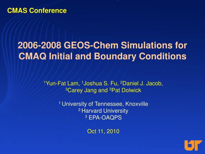
CMAS Conference. 2006-2008 GEOS-Chem Simulations for CMAQ Initial and Boundary Conditions. 1 Yun-Fat Lam, 1 Joshua S. Fu, 2 Daniel J. Jacob, 3 Carey Jang and 3 Pat Dolwick 1 University of Tennessee, Knoxville 2 Harvard University 3 EPA-OAQPS Oct 11, 2010. Outline of talk.

E N D
CMAS Conference 2006-2008 GEOS-Chem Simulations for CMAQ Initial and Boundary Conditions 1Yun-Fat Lam, 1Joshua S. Fu, 2Daniel J. Jacob, 3Carey Jang and 3Pat Dolwick 1 University of Tennessee, Knoxville 2 Harvard University 3 EPA-OAQPS Oct 11, 2010
Outline of talk • Background and Motivation • Long-range transport • Increase in background concentration • Development & Methodology • New CB05 with AE5 mapping table • Global and Regional Model Configurations • GEOS-Chem and CMAQ simulation • Sensitivity to Initial & Boundary Conditions • Conclusions
Why boundary condition is important to U.S. air quality? • Long-range transport of air pollutant 1 • Enhancement of background pollutants concentration 2 • The Canadian and Mexican pollution enhancement averages 3-4 ppb in the US in summer 3 • peaking at 33 ppb in upstate New York (on a day with 75 ppb total ozone) and 18 ppb in Canadian and Mexican pollution enhancement 1Heald, C.L., et al., J. Geophys. Res. (2003), Mian Chin, et al., Atmos. Chem. Phys. (2007) 2Vingarzan R., Atmos. Envir. (2004), Ordonex C., et al., Geophys. Res. L. (2007) 3Huiqun Wang, et al., Atmos. Envir. (2009), 43, 1310–1319
GEOS-Chem Simulations • 2005–2008 GEOS-Chem simulations • To study the inter-annual variability of boundary condition from each bound (North, East, South and West) • Propose a fixed domain for sharing CMAQ initial and boundary conditions using 34-layer IC/BC file • Study the impacts of using 24L IC/BC Vs. 34Lto24L • Identify the effects of this technique to CMAQ output.
GEOS-Chem v8-03-01 Domain: Globe Horizontal Grid Spacing: 2 ° x 2.5° Horizontal Coordinate: Lat x Lon Vertical Grid Spacing: 54 layers Simulation Period: 2005-2008 Meteorological Input: GEOS5 Global Model Configuration Emissions Summary
Inter-annual Variability of Ozone (Avg JFM) CMAQ BCON 10 ppb 9ppb
Inter-annual Variability of Ozone (Avg AMJ) CMAQ BCON All less than 5 ppb
Inter-annual Variability of Ozone (Avg JAS) CMAQ BCON All less than 5 ppb
Development of GEOS-Chem to CMAQ IC/BCs Module (Geo2CMAQ) • Newest version – 2010 (version 2.2) • Tropopause determining algorithm to remove stratospheric effects from GEOS-Chem • Update to the newest version of GEOS-Chem v8-03-01 • Add CB05-AE5 conversion table
Introducing the concept of tropopause • Imaginary layer that separates between stratosphere and troposphere. • Abrupt change of physical phenomenon • Three different ways to define tropopuase • Temperature1 (1937) => Thermal tropopuase • PV2 (1959) => Dynamical tropopause • Ozone3 (1995) => Ozone tropopause 1 1Stohl A., et al., J. Geophys. Res. (2003) 2Shapiro (1980), WMO (1986) 3Bethan, S., et al, J. R. Meteorol. Soc (1995)
July 25, 2002 (Trinidad Head, CA) (ppmv) CO Ozone Temp. Ozone Concentration (ppmv) (Degree C) Vertical Profile and Tropopause Determining Algorithm • Determining tropopause based on the dynamical searching on maximum rate of change of slope • Abrupt change of ozone and CO concentrations occurred • Each grid in downscaling has its own ozone tropopause height, so temporal and spatial integrity can be conserved…
Geo2CMAQ Conversion tool 3Lam, Y. F. and J. S. Fu (2009)., Atmos. Chem. Phys., 10, 4013-4031, doi:10.5194/acp-10-4013-2010
CB05-AE5 Conversion Table ??The ratio between Aged SOA and Non-aged SOA??
CMAQ Model Configurations CMAQ V4.7 • Meteorological Input MM5 V3.7 • Domain: CONUS • Horizontal Grid Spacing: 36 km • Horizontal Coordinate: LCC • Vertical Grid Spacing: 24 layers • Simulation Period: 2005 • IC/BC: GEOS-Chem 2005 Two IC/BC scenarios were performed: • 24 Layer IC/BC using 24-layer MCIP product • 24 Layer IC/BC using average layer collapsing technique from 34-layer MCIP & 34-layer IC/BC
24-layer Vs 34-layer (sample point) The major effect will be on 23rd and 24th layer
Comparison of “24L” – “24L=>34L” Surface Concentration JUL – O3 JAN – O3 JAN – SO2 JUL – SO2
Summary • The GEOS2CMAQ program improves the downscaling process for generating GEOS-Chem IC/BC. In this study, total of four years of GEOS-Chem simulation have been performed • The variability of average seasonal background boundary concentration of ozone is about 10–12 ppbv • Mostly occurred at the upper level of North and South bounds • The newt approach for generating the IC/BC using full sigma level gives a better data portability. It also makes it easier to share IC/BC data with other researchers. • Only required very limited processing. • It only changes the surface ozone level by less than 0.25 ppb from original method. • We are in the progress to construct a website to share the IC/BC files, which we have on those 4 years.
Acknowledgement • USEPA’s STAR and GCAP (phase 1 and phase 2) funding supports
Q & A Thank you!