Download
1 / 49
580 likes | 850 Views
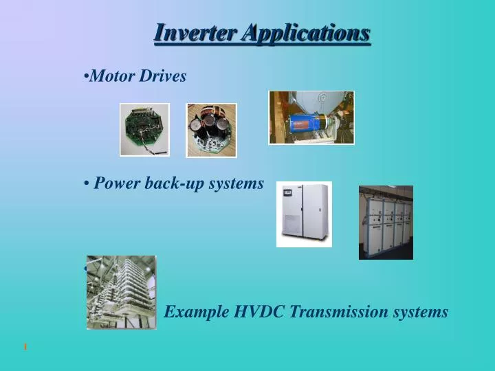
Inverter Applications. Motor Drives Power back-up systems Others: Example HVDC Transmission systems. Single Phase Inverter Square-wave “Modulation” (1). V dc. v out (t). t. -V dc. Single Phase Inverter Square-wave “Modulation” (2). THD = 0.48.

E N D
Inverter Applications • Motor Drives • Power back-up systems • Others: • Example HVDC Transmission systems
Single Phase Inverter Square-wave “Modulation” (1) Vdc vout(t) t -Vdc
Single Phase Inverter Square-wave “Modulation” (2) THD = 0.48 Characteristics: - High harmonic content. - Low switching frequency. - Difficult filtering. - Little control flexibility.
Single Phase Inverter Square-wave “Modulation” (3) Vdc vout(t) t -Vdc
Single Phase Inverter Square-wave “Modulation” (4) Example with Vout-1=1.21Vdc THD = 0.3 Characteristics: - High harmonic content. - Low switching frequency. - Difficult filtering. - More control flexibility.
Single Phase Inverter Pulse Width Modulation (1) D is the duty cycle of switch Q1. D is the portion of the switching cycle during which Q1 will remain closed. In PWM D is made a function of time D=D(t)
Single Phase Inverter Pulse Width Modulation (2) Modulation function • Let’s where Modulation index Fundamental Signal
Single Phase Inverter Pulse Width Modulation (3) Moving average t
Single Phase Inverter Pulse Width Modulation (4) Implementation issue: time variable “t” needs to be sampled. Two basic sampling methods: UPWM NSPWM
Single Phase Inverter Pulse Width Modulation (5) t
Single Phase Inverter Pulse Width Modulation (6) Considering that
Three Phase Inverter Pulse Width Modulation (1) Active States: Zero States:
Three Phase Inverter Pulse Width Modulation (2) Modulation Functions “Zero-Sequence” Signals
Three Phase Inverter Pulse Width Modulation (3) Triplen Harmonics (3, 9, 15, …) Fundamental Signal Modulation index Other Harmonics (5, 7, 11, 13, 17, ….)
Three Phase Inverter Pulse Width Modulation (4) t
Classic Approaches to PWM (1) Time Domain Use of modulation signal: Duty cycle computation: t Sector limits
Classic Approaches to PWM (2) Classic SVM - Application Park’s Transformation Park’s Transformation 3 2 - d-PI Controller Domain Transformer (Modulator) + Space Vector - Time q-PI Controller + Switch Control DC Source Inverter Motor (From Vector Controller) Disadvantages: Can’t see evolution in time Loss of information about e0-3(t)
Classic Approaches to PWM (3) Classic SVM Space vector domain SECTOR II SECTOR I SECTOR III 2 Bases SECTOR IV SECTOR VI BSVM changes in each sector SECTOR V BSVM in sector I In O:
Classic Approaches to PWM (4) Classic SVM Transitions within sector I T7=T0 S6 S2 SVM Computation S4 • Track the sector in which is in and based on it select the appropriate set of basis Bij • Calculate the coordinates of in the basis Bij • - Change the coordinates of the reference voltage vector S7 S3 S0 S5 S1 from basis Bdq to basis Bij. The sector dependant transformation yields the period of time Ti that the machine remains in each state in a given sampling period. - When the time Ti is finished move to the next state following the sequence given by the SVM state machine.
Mathematical Framework (1) Complete representation involves a 3-D space Then, a 3-D vector can be introduced: Control Time Domain Space Vector Domain Output Time Domain
Mathematical Framework (2) Control Time Domain Functions of time are used as basis
Mathematical Framework (3) Space Vector Domain When e0-H(t)=0, describes a circumference with radius equal to m.
Mathematical Framework (4) Output Time Domain
Mathematical Framework (5) Output Time Domain Length of sides equal to 2 Each corner represents one state State sequence is obtained naturally Balanced system plane Sectors: six pyramid-shaped volumes bounded by sides of the cube and |vi|=|vj| planes (i, j = a,b,c; i j).
Mathematical Framework (6) Matrix R When e0-H(t)=0, describes a circumference with radius equal to m. 1st Idea: Use Park’s transformation to a synchronous rotating reference frame: Instantaneous values of the voltages
Mathematical Framework (7) Matrix R Problem: components in and are constant values I am interested in having a constant value in 2nd Idea: Freeze the rotational reference frame at t=0
Mathematical Framework (8) Matrix R 3rd Idea: Rearrange the product.
Mathematical Framework (9) Matrix R 4th Idea: Eliminate the dependency on e0-3(t) in order to have a constant coordinate in
Mathematical Framework (10) Matrix R In order to include e0-H(t) we need to follow the same steps and apply superposition.
Mathematical Framework (11) Matrix W W’
Mathematical Framework (12) Matrix W • Take the transpose • and apply scaling • factor • Include e0-3(t) in • order to have it as • a component
Mathematical Framework (13) Matrix S S=WR
3D Analysis and Representation SVM UPWM
3D Analysis and Representation 3D Representation: Plot evolution of in output time domain during a complete fundamental period. The resulting curve always lays within the cube defined by the switching states.
3D Analysis and Representation Triplen harmonic distortion: Evolution away from the plane va+vb+vc=0 Other harmonic distortion: non circular projection of the curve over the plane va+vb+vc=0 Sharp corners indicate the presence of higher order harmonics.
Commonly used schemes SVM Square wave
3D Analysis and Representation Square wave
3D Analysis and Representation Phase and Line Voltages (1)
3D Analysis and Representation Phase and Line Voltages (2) voa (t) va (t) Direction of vab t Direction of voa
3D Analysis and Representation Phase and Line Voltages (3) voa (t) va (t) t
3D Analysis and Representation Maximum non distorting range Radius of circle is m if it is measured in the Space Vector Domain. There is a scaling factor in W
3D Analysis and Representation If fswitch>>ffund then
3D Analysis and Representation Sector II Sector III Sector I T7 T6 T4 T0 T7 T6 T2 T0 T7 T3 T2 T0 Qa Qb Qb Qb Qa Qc Qc Qc Qa
Analysis of SVM (1) T7=T0 Dmin=1-Dmax vmax +vmin=0 S is sector dependent (considering e0-H(t)=0) SVM tends to approximate the trajectory of a square wave, but adds 3rd harmonic and higher order triplen harmonics No difference in sequence compared to other schemes
Analysis of SVM (2) t t Fundamental and zero-sequence signal Modulating signals
Analysis of SVM (3) Control Time Domain Space Vector Domain Output Time Domain Digital implementation related to sampling method selected, not to the modulation function used.