Download
1 / 25
250 likes | 261 Views
Issues on Graph Plotting in the A-level Biology Examinations. Dr. W.K. Yip Botany, HKU. Background. In 1997 AL Biology paper 1B Q12, it was demanded that the growth curves of this question must be drawn by a series of straight lines in order to see the different growth patterns of cows.

E N D
Issues on Graph Plotting in the A-level Biology Examinations Dr. W.K. Yip Botany, HKU
Background • In 1997 AL Biology paper 1B Q12, it was demanded that the growth curves of this question must be drawn by a series of straight lines in order to see the different growth patterns of cows. • In a TAS teachers’ meeting held in 1998, different opinions concerning the graph presentations on the water potential experiment using potato tissue. • Seemingly dual standards/ or contradictory standards of HKEA?
Issues to be clarified • Does the way to joint data points in a graph constitute an interpretation of the data set? • When to join data points with a smooth curve or a series of straight lines. • What are smooth curves/ lines of best fit?
1997 Examiner’s report on Q12 • The line on a graph is referred to as a curve even though the line is a straight line. • A curve can be in the form of a smooth line, a best straight line through the points, or in the form of a series of straight lines joining successive points. • In the former two cases, the curves are drawn as such only if there are good reasons to think that the intermediate values would fall on the curve, otherwise a series of straight lines joining the points indicates that the values between the recorded points are not known.
Using a curve in a graph to estimate unknowns : regression of data points Not correct Correct (linear regression) Correct (polynomial regression)
Tabulated data YES Histogram YES Frequency table Are data grouped in some way? Both sets of data numeric? Bar chart NO Was one factor manipulated in the experiment? NO Plot scatter diagram YES Responding variable Manipulated variable y Plan-a-graph Modified from D. Marshall “Inquiry and Investigation in Biology: An Introduction.” ABAL Unit One, Cambridge University Press, 1983 x Set scales and origin, plot points, label and title Join points with short straight lines NO Points or theory indicate smooth change? Are there large jumps between points? Plot log-linear or log-log graphs YES YES OPTIONAL Draw curve or line of best fit
Curves with theories Normal distribution curve Sigmoid curve Saturation kinetic curve Exponential curve
Mean body weight (kg) Day 1 Day 20 Day 40 Day 60 Group A cows (fed with sterilized grass) 800 780 748 680 Newborns of Group A (fed with milk from parent) 60 68 92 108 Group B cows (fed with unsterilized grass) 800 856 912 968 Newborns of Group B (fed with milk from parent) 60 68 100 140 1997 AL Biology exam paper 1B Question 12 Changes of cow body weight as affected by diet
Cows fed with un- Sterilized grass (Gp B) Cows fed with Sterilized grass (Gp A) Newborns from Gp B Newborns from Gp A
Treatment with different concentrations of sucrose solution (M) 0 0.2 0.4 0.6 0.8 1.0 Initial length of potato cylinder (cm) 3 3 3 3 3 3 Final length of potato cylinder (cm) 3.40 3.20 3.05 2.95 2.90 2.90 Change in length of potato cylinder (cm) +0.4 +0.2 +0.05 -0.05 -0.1 -0.1 % change in length +13.3 +6.7 +1.7 -1.7 -3.3 -3.3 Water Potential of Potato Tissue: Data Set A
Concentrations of sucrose solution (M) 0 0.1 0.2 0.3 0.4 0.5 0.6 0.7 0.8 0.9 1 Initial weight (g) 0.792 0.777 0.780 0.744 0.748 0.762 0.806 0.808 0.793 0.817 0.800 Final weight (g) 0.928 0.878 0.804 0.749 0.702 0.707 0.678 0.652 0.623 0.617 0.592 Change in weight (g) + 0.136 + 0.101 + 0.024 + 0.005 - 0.046 - 0.055 - 0.128 - 0.156 - 0.170 - 0.200 - 0.208 % Change + 17.2 + 13.0 + 3.1 + 0.7 - 6.1 - 7.0 - 15.9 - 19.3 - 21.4 - 24.4 - 26.0 Water Potential of Potato Tissue: Data Set B
Point Polynomial Data Regression: Data Set B (% Change) 0.29M
Concentrations of sucrose solution (M) 0 0.1 0.2 0.3 0.4 0.5 0.6 0.7 0.8 Initial length (cm) 3.00 3.00 3.00 3.00 3.00 3.00 3.00 3.00 3.00 Final length (cm) 3.25 3.20 3.10 3.05 3.05 3.00 3.00 2.95 2.90 Change in length (cm) + 0.25 + 0.20 + 0.10 + 0.05 + 0.05 - 0 - 0 - 0.05 - 0.1 % Change + 8.3 + 6.7 + 3.3 + 1.7 + 1.7 - 0 - 0 - 1.7 - 3.3 Water Potential of Potato Tissue: Data Set C
Data Point Distribution : % Change vs Sucrose concentrations of all three sets of data
Conclusion • The ways in which the data points should be joined should be considered on a case by case basis which indicated the interpretation of the writer or the usage of the curve.