Download
1 / 38
380 likes | 390 Views
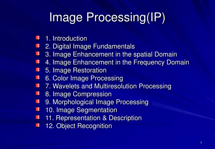
Image Processing(IP). 1. Introduction 2. Digital Image Fundamentals 3. Image Enhancement in the spatial Domain 4. Image Enhancement in the Frequency Domain 5. Image Restoration 6. Color Image Processing 7. Wavelets and Multiresolution Processing 8. Image Compression

E N D
Image Processing(IP) • 1. Introduction • 2. Digital Image Fundamentals • 3. Image Enhancement in the spatial Domain • 4. Image Enhancement in the Frequency Domain • 5. Image Restoration • 6. Color Image Processing • 7. Wavelets and Multiresolution Processing • 8. Image Compression • 9. Morphological Image Processing • 10. Image Segmentation • 11. Representation & Description • 12. Object Recognition
Introduction • 1.1 What is Digital Image Processing • 1.2 The Origins of Digital Image Processing • 1.3 Examples of Field that Use Digital Image Processing • 1.4 Fundamental Steps in Digital Image Processing • 1.5 Components of an Image Processing System • 1.6 Importance Academic IP Journals Research • 1.7 Course Requirements
1.1 What is Digital Image Processing • 1. Related Terminologies • a. image ---- still • b. picture --- image • c. graph ----- conceptual • d. pattern --- conceptual • e. graphics -- drawings • f. animation - dynamic graphics • g. video ------ dynamic images
1.1 What is Digital Image Processing • 1. Image ( monochrome image ) • 2-D light intensity function f(x,y) • where (x,y): spatial coordinates; • value of f : brightness of gray level at (x,y) • 2. Digital Image • image discretized both in spatial and gray levels • 3. Image Elements • picture elements (pixels or pels)
1.1 What is Digital Image Processing • 4. Related Fields • a. computer vision (CV) ----------- 3-D IP • b. signal processing (SP) ---------- 1-D IP • c. computer graphics (CG) -------- generation of drawings • d. image synthesis (IS) ------------ generation of images (IP + CG ) • e. pattern recognition (PR) ------- theory • f. scientific visualization (SV) --- application of IS • g. multimedia technologies ------- application of a thru f
1.1 What is Digital Image Processing • Three types of computerize processes: • Low-level processes: • Primitive operations such as : image processing to reduce noise, contrast enhancement, and image sharpening. • Both its inputs and outputs are images • Mid-level processes: • Segmentation ( partitioning an image into regions or objects) • Description of those objects to reduce them to a form suitable for computer processing, • Classification ( recognition) of individual objects. • Its inputs generally are images, but its outputs are attributes extracted form those image • High-level processes: • “Making sense” of an ensemble of recognized objects
1.2 The Origins of Digital Image Processing • 1. Improving digitized newspaper in 1920s to 1950s
1.2 The Origins of Digital Image Processing • 2. Improving images from space programs from 1964
1.2 The Origins of Digital Image Processing • 3. From 1960s till now, the IP field has grown vigorously • 4. Computer tomography(CT) • an important achievement of in medicine ( has won a Nobel Prize)
1.3 Examples of Field that Use Digital Image Processing • 1.3.1 Gamma –Ray Imaging
1.3 Examples of Field that Use Digital Image Processing • 1.3.2 X-ray imaging
1.3 Examples of Field that Use Digital Image Processing • 1.3.3 Imaging in the Ultraviolet Band
1.3 Examples of Field that Use Digital Image Processing • 1.3.4 Imaging in the Visible and Infrared Bands
1.3 Examples of Field that Use Digital Image Processing • 1.3.4 Imaging in the Visible and Infrared Bands
1.3 Examples of Field that Use Digital Image Processing • 1.3.4 Imaging in the Visible and Infrared Bands
1.3 Examples of Field that Use Digital Image Processing • 1.3.4 Imaging in the Visible and Infrared Bands
1.3 Examples of Field that Use Digital Image Processing • 1.3.4 Imaging in the Visible and Infrared Bands
1.3 Examples of Field that Use Digital Image Processing • 1.3.4 Imaging in the Visible and Infrared Bands
1.3 Examples of Field that Use Digital Image Processing • 1.3.4 Imaging in the Visible and Infrared Bands
1.3 Examples of Field that Use Digital Image Processing • 1.3.4 Imaging in the Visible and Infrared Bands
1.3 Examples of Field that Use Digital Image Processing • 1.3.5 Imaging in the Microwave Bands
1.3 Examples of Field that Use Digital Image Processing • 1.3.6 Imaging in the Radio Bands
1.3 Examples of Field that Use Digital Image Processing • 1.3.6 Imaging in the Radio Bands
1.3 Examples of Field that Use Digital Image Processing • 1.3.7 Examples in which Other Imaging Modalities Are Used
1.3 Examples of Field that Use Digital Image Processing • 1.3.7 Examples in which Other Imaging Modalities Are Used
1.3 Examples of Field that Use Digital Image Processing • 1.3.7 Examples in which Other Imaging Modalities Are Used
1.3 Examples of Field that Use Digital Image Processing • 1.3.7 Examples in which Other Imaging Modalities Are Used
1.6 Important Academic IP Journals • 1. IEEE Transactions on Pattern Analysis. & Mach. Intelligence • 2. IEEE Transactions on Systems, Man, and Cybernetics • 3. IEEE Transaction of Image Processing • 4. Computer Vision, Graphics, and Image Processing • 5. Pattern Recognition • 6. Image and Vision Computing • 7. International Journal of Computer Vision • 8. Machine Vision and Applications • 9. Pattern Recognition Letters
1.7 Course Requirements • 1. Textbook: • R.C.Gonzalez and R.E. Woods, Digital Image Processing, Addison-Wesley Pub. Co., Readings Massachusetts, USA, • 2. Grade Evaluation: • b. one or two exams • a. about 3~4 homeworks • 3. Pre-requistes • Ability of programing or Experience of IP Software ( MATLAB).
2.4 Some Basic Relations Between Pixels • 2.4.1 Neighborhood of a Pixel • 1. Given a pixel p in the center of 9 • pixels: • a b c • d p e • f g h • then • 4-neighbors of p = b, d, e, g; • 8-neighbors of p = a, b, c, d, e, f, g, h; • diagonal neighbors of p = a, c, f, h;
2.4 Some Basic Relations Between Pixels • 2.4.2 Connectivity • 1. Terms: 4-connected , 8-connected , 4-adjacent , 8-adjacent , path connected. • 2. Connected component (c. c.): • for any pixel p in a set of pixels S , the set of pixels MS that are connected to p is a c.c. of p S c.c.
2.4 Some Basic Relations Between Pixels • 2.4.3 Labeling of Connected Components • 1.Gives a pixel p with r and t as its upper and left-hand neighbors as follows: • r • t p • then the following algorithm labels all c.c. in an binary image ( This algorithm for 4-connected) • a. Scan the image from left to right and from top to bottom; • b. If p = 0 , continue the scan; • c. If p = 1 , exam r and t; • if r = t = 0 assign a new label to p;
2.4 Some Basic Relations Between Pixels • if r = 1 & t = 0 , assign the label of r to p; • if r = 0 & t = 1 , assign the label of t to p; • if r = t = 1 & labels of r & t identical, then assign that label to p; • if r = t = 1 & labels of r & t different, then assign one of the labels to p and make the two labels “equivalent”; • d. Sort all the equivalent label pairs into equivalent classes, and assign a distinct label to each class. • 2.Do a second scan thru the image and replace each label by the label assigned to its equivalent class. • 3. For sorting of equivalent labels ,see Section 2.4.4 • *P.S. The above is for 4-connectivity, another algorithm in textbook for 8-connectivity;
2.4 Some Basic Relations Between Pixels • 2.4.4 Relations , Equivalence , and Transitive Closures • 1. A property : • If R is an equivalent relation on a set A , then A can be divided into a group of disjoint subsets , called equivalent classes , such that aRb iff a and b are in the same subset.
2.4 Some Basic Relations Between Pixels • 2.4.5 Distance Measures • 1. Given three pixels p, q, and z with coordinates (x, y), (s, t), (u, v), respectively, we have the following three types of distances: • a. Euclidean distance • De(p, q) = [(x-s)2+(y-t)2]1/2 • b. City-block distance • D4(p, q) = | x - s | + | y - t | • The pixels with D4=1 to a pixel p are the 4-neighbors of p • c. Chessboard distance • D8(p, q) = max ( | x - s | , | y - t | ) • The pixels with D8=1 to a pixel p are the 8-neighbors of p
2.4 Some Basic Relations Between Pixels • 2.4.6 Arithmetic/Logic Operations • 1. Mask operations • are arithmetic/logic operation applied to the neighborhood ( with g. l. z1, z2, …….., z9) of a pixel with g. l. z5, e.g., • z5 z=(z1+z2+z3…….+z9)/9 • 2.Notes: • a. g. l. = gray level; • b. Masks are also called templates, windows, filters, etc. • 2.5 Image Geometry ( see the textbook) • 2.6 Photographic Films ( see the textbook).