Download
1 / 50
500 likes | 709 Views
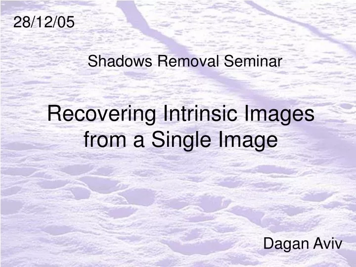
Recovering Intrinsic Images from a Single Image. Shadows Removal Seminar. 28/12/05. Dagan Aviv. Relies on:.

E N D
Recovering Intrinsic Imagesfrom a Single Image Shadows Removal Seminar 28/12/05 Dagan Aviv
Relies on: • Marshall F. Tappen, William T. Freeman and Edward H. Adelson.“Recovering Intrinsic Images from a Single Image.”IEEE Transactions on Pattern Analysis and Machine Intelligence, vol. 27, no. 9, pp. 1459-1472, September, 2005 • Matt Bell and William T. Freeman.“Learning Local Evidence for Shading and Reflectance”Proc. Int’l Conf. Computer Vision, 2001.
Motivation • Interpreting real-world images • Distinguish the different characteristics of the scene • Shading and reflectance – two of the most important characteristics
Short Introduction • Image is composed of Shading Intrinsic and Reflectance Intrinsic images
Our Goal • Decompose an Input Image into its Intrinsics • Simple Approaches like Band Filtering won't help us. for example:
Our Approach • Recovering the images using multiple cues • Implicit assumption – surfaces are lambertian (a good starting point…) • Classify Image Derivatives
Separating Shadows and Reflectance • As shown in the preceding talk: • Recovering S and R using derivatives of the input image I
Creating The Intrinsic Image • Building S and R is performed in the same manner as shown in the last talk (Weiss) - convolution operator imgX - S or R F – estimated derivative f – derivative filter – ([-1 1] in out case) f(-x,-y) – reverse copy of f(x,y)
Binary Classification • Assumption – each derivative is caused either by Shadings or Reflectance • This reduces our problem into a binary classification problem
Classifying Derivatives • 3 Basic phases: 1. Compute image derivatives 2. Classify each derivative as caused by shading or reflectance 3. Invert derivatives classified as shading to find shading images. The reflectance image is found in the same way.
Classifying Derivatives • The Classifying stage is achieved using two forms of local evidence:1. color information2. statistical regularities of surfaces (Gray-scale information)
Color Information • When speaking of defusive surfaces : And lights have the same color,changes due to shading should affectR,G and B proportionally
Color Information • Let and be RGB vectors of two adjacent pixels. • A change due to shading can be represent as:α is scalar (intensity change)
If - shading Else - reflectance Color Information • If the changes are caused by a reflectance change • After normalizing and , the dot product will result 1 if the changes are due to shadings ( ) • Practically a threshold is chosen manuallyso:
Color Information • The threshold eliminates chromatics artifacts caused by JPEG compression for example • The chosen threshold: cos 0.01 • When speaking of non-lambertian surfaces: the results are less satisfying
Color Information - examples Input Image Shading Image reflectance Image
Color Information - examples Black on white may be interpreted as intensity change. Resulting in misclassification
Color Information - examples As before - the face is incorrectly placed in the shadings image The hat specularity is added to the reflectance image
Gray-scale Information • Shading patterns have a unique appearance • We will examine ROIs wrapping each derivative in a gray-scale image to find shadow patterns
Gray-scale classifier • The Basic Featurewhere I is the ROI (patch) surrounding a derivative and w is a linear filter • the non-linear F is the result in the center of the ROI
Training the classifier • Two tasks are involved: 1. choosing the filters set – which will build the features 2. training the classifier on the features
AdaBoost (in general) • Both Tasks are achieved by the chosen classifier – AdaBoost • First introduced in 1995 by Freund and Schapire • The main idea is to boost a “weak classifier” – a classifier with error slightly less than 0.5
AdaBoost • The classifier is trained by giving it a training set • is a binary mapping from the X domain to the Y domain – {-1,+1} • In our case X is a set of synthetic images of shadings and reflectance,-1 is for reflectance and +1 is for shading
AdaBoost • AdaBoost is also gets the weak classifier as an input • The learning stage is iterative • At each round t, AdaBoost weights the training set and run the weak classifier • The weak classifier job is to find an hypothesis h such that:
AdaBoost • Elements that were misclassified will get a higher weight for the next iteration • AdaBoost also weights the classifier votes • At the end – once the desired number of rounds has run, all the weighted votes is gathered to compute the final strong classification H.
AdaBoost – toy example • Original Training Set
AdaBoost – toy example Round 1
AdaBoost – toy example Round 2
AdaBoost – toy example Round 3
AdaBoost – toy example Final result
AdaBoost – matlab source • See the next archive for AdaBoost Matlab implementation (and more)
If otherwise Our AdaBoost • The Weak Classifierwhere andrecall that
Our AdaBoost • So AdaBoost needs to choosews, thresholds and s • w – a set of patches constructed from 1st and 2nd derivatives of Gaussian filters • The training set (which the I’s patches is derived from) is a set of synthetic images
Our AdaBoost • The training set is evenly divided between shading:and reflectance:
Our AdaBoost • The shading images were lit from the same direction • An assumption – when an input image is given, the light direction is known • Preprocess - rotate the input image so the light will match the light in the training set
GrayScale Information - examples The shading image is missing some edges These edges didn”t appear in the training set
GrayScale Information - examples Misclassification of the cheeks – due to weak gradients
Combing Informations • The final result is based on a statistical calculation of conditional probability • Assumption: both classifiers (color and gray-scale) are statistically independent • Bayes rule: • Each Pr is computed with some modifications on the classifiers
Handling Ambiguities • Ambiguities - In the former slide for example – the center of the mouse Shading example Input image Reflectance example
Handling Ambiguities • Derivatives that lie on the same contour should have the same classification • The mouth corners are well classified as reflectance
Handling Ambiguities • Areas where the classification is clear are to propagate their classification to disambiguate other areas • Achieved by a Markov Random Field – which generalize Markov Chains
Handling Ambiguities • First a potential function is applied on the image finding the “most interesting” gradients • Then the propagation starts from points having both strong derivatives and no ambiguities
The End Thank you