Download
1 / 44
440 likes | 557 Views
Chapter 11: Selected Quantitative Relationships (pt. 1). ISE 443 / ETM 543 Fall 2013. The development of large, complex systems involves the use of quantitative relationships. To predict system performance before it is built response times success rates system availability

E N D
Chapter 11: Selected Quantitative Relationships (pt. 1) ISE 443 / ETM 543 Fall 2013
The development of large, complex systems involves the use of quantitative relationships • To predict system performance before it is built • response times • success rates • system availability • system reliability • error rates • catastrophic failure • Because of the uncertainty involved, probability is the most used quantitative relationship in systems engineering (and, to a lesser extent, project management)
To start, we’ll review the fundamentals • Basic probability – Ned and Ryan S. • Discrete distributions • binomial distribution – Lexie and Rebecca • poisson distribution – Filipe, Xin, and Yuan • Continuous distributions • normal distribution – Alfred and James • uniform distribution – Justin and Gleidson • exponential distribution – Elvire and Ryan K. • Means and variances – Jamie and Geneve • Sums of variables – Isis and Jessica • Functions of random variables – Charmaine and Melanie • Two variables (joint probability) – Celso and David • Correlation – Lucas and Kyle
Your turn … • Form into pairs. As a pair review the list on the previous slide and select a topic you wish to review for the class. • You may want to have at least one “backup” topic. • Once you have decided on a topic, STAND UP. When you are recognized (I will go in order) state your selected topic. • If someone else selects your topic, move to your “backup”. If you don’t have a backup, sit down until you have selected another. • Review the section in the book related to your topic and develop a brief summary to share with the class today (you will have 10 minutes to prepare). • 10 minutes after the last topic is selected, we will go through each topic as a class and discuss what you have so far. • Make note of the feedback you receive. You may find this useful when completing the homework assignment.
For any given event P > 0 For a certain event, P = 1, if it can’t happen P=0, if it may happen it’s between 0 and 1. If 2 events are mutually exclusive, add the probabilities to find the probability of either one happening To find probability of BOTH happening, multiply the 2 probabilities Other rules for independence, non-independent, etc. Basic probability
Basic Probability For any event, the possibility of it occurring is greater than or equal to zero. If it’s certain to happen, the probability of it occurring is 1. If it’s completely impossible, the probability of it occurring is 0. Anything else has a probability of between 1 and 0. For example, if you roll a dice there is a 1/6 probability of getting any particular number To find the probability of at least one of two mutually exclusive events happening, add the odds together. For example, if you roll a dice there is a 1/6 chance to get a 5 and a 1/6 chance to get a 4. Therefore, there is a 2/6 (1/3) chance of getting either a 5 or a 4. By Ryan Stapleton and Ned Nobles
If you want to get both of two possibilities, multiply the odds together. For example, if you roll 2 dice, the odds of getting a 5 and a 4 are 1/6 *1/6, or 1/36. By Ryan Stapleton and Ned Nobles
Arises when there are repeated independent trials with only 2 possible results If P(success) = p and P(failure) = q, then p+q=1 The distribution is the equation 11.23 on page 345. The distribution defines the probability of exactly x successes in n independent trials Example at top of page 346 Discrete distributions: Binomial
Binomial Distribution Arises with repeated independent trials with only two possible outcomes P(success)=p P(failure)=q p+q=1 , for x= 0,1,2,3,…n , otherwise The distribution defines the probability of exactly x successes in n independent trials Lexy Blaha & Rebecca King
Example If, when throwing a die, an odd number is success and an even number failure, the probability of exactly 4 success in 10 trials is P(4)= =.205 Lexy Blaha & Rebecca King
Real World Example In a multiple-choice exam with 4 choices for each question, what is the probability that a student gets exactly 2 correct if he chooses the answers randomly. Assume there are 10 questions in all. n= 10 p= 1/4 = 0.25 We want P(x = 2 ) , where x is the number of correct answers out of 10. = 0.2816 Mean = np = 10(1/4) = 2.5 Standard deviation = = 1.3693 Lexy Blaha & Rebecca King
Deals with the issue of software reliability May be used in situations for which events happen at some rate and we wish to ascertain the probability Example on page 346 Formula is also on 346 Discrete distributions: Poisson
The Poisson Distribution • The Poisson is a discrete distribution given by the following formula: • P(k) = • Where P(k) is the probability of exactly k events of interest, is the rate at which such events are occurring, and t is the time over which the events are occurring. Team: Xin, Yuan, Filipe
The Poisson Distribution • The distribution may be used in situations for which events happen at some rate and we wish to ascertain the probability of some number of events occurring in a total period of time, or in a certain space. Team: Xin, Yuan, & Filipe
Example Cars are passing a toll booth at an overall rate of about 120 cars per hour. The probability that exactly three cars will pass through the toll booth in a period of 1 minute would be P(3) = = 0.18 Team: Xin, Yuan, & Filipe
AKA Gaussian Bell-shaped curve Density function on page 347, eq. 11.25 Integrate (p(x < X)) OR use tables (p(z <Z)) Continuous distributions: Normal
Normal Distribution • Gaussian Distribution • To calculate probabilities, one must integrate the density function • This calculates the probability that x is less than or equal to a specified number • However, normal distribution is not readily integrable so we must resort to using a Z-table. Albert Sykes & James Edwards
Z-Table Albert Sykes & James Edwards
Example Albert Sykes & James Edwards
Occurs when there is a constant probability over a range Cumulative density function is a triangle from 0 to 1. Equations for the mean and variance are on page 350 Example on page 350 (arrow shot at bullseye) Continuous distributions: Uniform
Uniform Distribution Source: http://www.giackop.com/blog/wp-content/uploads/numbers.jpg The Uniform Distribution is useful in random number generation. Random Numbers are very useful in: gambling statistical sampling, cryptography, and anything seeking an unpredictable result. Justin Blount - GleidsonGurgel - ISE 443 Project Management
Uniform Distribution http://upload.wikimedia.org/wikipedia/commons/thumb/9/96/Uniform_Distribution_PDF_SVG.svg/350px-Uniform_Distribution_PDF_SVG.svg.png upload.wikimedia.org/wikipedia/commons/thumb/6/63/Uniform_cdf.svg/350px-Uniform_cdf.svg.png Its graph is ‘flat’ over its entire range. Mean: (a+b)/2 Variance: (b-a)^2/12 PDF: CDF: Justin Blount - GleidsonGurgel - ISE 443 Project Management
Uniform Distribution • Applications: • Statistics: • Randomness is commonly used to create simple random samples. This lets surveys of completely random groups of people provide realistic data. • Computer Simulation: • Simulation of random events require random numbers. • Gambling: • Gambling theory is based on random numbers. Justin Blount - GleidsonGurgel - ISE 443 Project Management
Density and cumulative dist function are illustrated on pg 350 The CDF starts at 0 and approaches 1 asymptotically Formulas are given on pg 350 Widely used in reliability theory wherein the value of lambda is taken to be a constant failure rate Failure rate and MTBF are reciprocals of each other Continuous distributions: Exponential
The Exponential Distribution • a.k.a radical exponential distribution, it is the probability distribution that describes the time between events in a Poisson process • The probability density function (pdf) of an exponential distribution is: • p(x)= λe-λx , for x ≥ 0 • = 0 , for x < 0 • The cumulative distribution function (cdf) starts at zero and approaches the value of unity asymptotically Elvire Koffi Ryan King
The Exponential Distribution • The cumulative distribution function is given by: • F(x) = 1 – e-λx , for x ≥ 0 • = 0 , for x < 0 • The exponential distribution is widely used in reliability theory wherein the value of λ is taken to be a constant failure rate for a part of a system • The failure rate and the mean time between failures (MTBF or 1/λ) are reciprocals of one another Elvire Koffi Ryan King
The Exponential Distribution • Example • Suppose that the amount of time one spends in a bank is exponentially distributed with mean 10 minutes, λ = 1/10. What is the probability that a customer will spend more than 15 minutes in the bank? • Solution: • P(x > 15) = e-15λ = e-3/2 = 0.22 Elvire Koffi Ryan King
Mean equation is on pg 340 (both discrete and continuous) Example of rolling dice Variance eq on pg 341 Variance indicates the spread of the distribution Std deviation is the square root of the variance A critical performance measure is the S/N ratio, which is … Means and variances
Mean Value (pg.340) • The mean value of rolling a single die is: • X=1(1/6)+2(1/6)+3(1/6)+4(1/6)+5(1/6)+6(1/6) • X=3.5 • Note-This result leads to a mean value that is different from all possible values of the variable. Duffy & Lopez Discrete: X = m(X) = ΣX P(X) for all X Continuous: x = m(x) = x p(x)dx EXAMPLE:
Variance and StandardDeviation (pg.341) • The variance of rolling a single die is: • σ2=(1-3.5)2(1/6)+(2-3.5)2(1/6)+…+(6-3.5)2(1/6) = 2.9 STANDARD DEVIATION • The square root of the variance √σ2 =σ • EXAMPLE: • Also known as the root-mean-squared: • √σ2= √2.9 = 1.7029 Duffy & Lopez VARIANCE Discrete: σ2 =Σ(X-m)2 P(X) for all X Continuous: σ2 = (x-m)2 p(x)dx EXAMPLE:
Signal-to-Noise Ratio (pg. 341) http://www.dspguide.com/ch25/3.htm Duffy & Lopez This is a ratio of the signal power over the noise power: S/N Equivalent to the square of the signal value to the variance of the noise distribution. EXAMPLE: This statistic can be related to classify accuracy given in an ideal linear discrimination, such as the human eyes ability to detect color signals.
Probability of the sum = sum of the probabilities (when the variables are mutually exclusive) Eq on pg 341 Distribution of the sum is the convolution of the individual distributions Variance of the sum is the sum of the variances only when the individual distributions are independent The mean value of the sum is the sum of the mean values Sums of variables
Sums of variables • If A and B are mutually exclusive, then: • P(A or B) = P(A +B) = P(A) + P(B) • The distribution of a sum is the convolution of the individual distributions • The sum of 2 uniform distributions lead to a triangular distribution • The mean value of a sum is the sum of the mean values: • Mean(Z) = E(Z) = mean(X + Y) = mean(X) + mean(Y) • The variance of a sum is the sum of the variances, only if the individual distributions are independent. That is, only when P(XY) = G(X)H(Y). • σ²(Z) = σ²(X + Y) = σ²(X) + σ²(Y) when X and Y are independent
Arise when we make a functional transformationa dn wish to examing the result Value is to track how a varaible behaves as it is processed through a system Example on pg 343 Functions of random variables
Functions of Random Variables One of the values of understanding the transformation of random variables (x) is to track how such a variable behaves as it is processed through a system (y) (pg. 344) In terms of y = mx+b, it is important to look at x because the input, in conjunction with the constants (m & b), determines the output (y) and its behavior From a Systems Engineering and Project Management standpoint, it is important to realize how the input variable (x), reacts with the constraints of the system to produce an output (y). Markman and Robinson
Functions of Random Variables Example Consider a random roll of two dice. There we defined the random variable X to represent the sum of the values on the two rolls. Now let h(x) = |x-7|, so that h(x) ≡ |X-7| represents the absolute difference between the observed sum of the two rolls and the average value 7. Then h(X) has a pmf on a new probability space S2 ≡ {0, 1, 2, 3, 4, 5}. In this case we get the pmf of h(X) being ph(x) (k) ≡ P(h(X) = k) ≡ P({s S: h(X(s)) = k}) for k S2 where, ph(x)(5) = P(h(X) = 5) ≡ P(|X-7| = 5) = 2/36 = 1/18 ph(x)(4) = P(h(X) = 4) ≡ P(|X-7| = 4) = 4/36 = 2/18 ph(x)(3)= P(h(X) = 3) ≡ P(|X-7| = 3) = 6/36 = 3/18 ph(x)(2) = P(h(X) = 2) ≡ P(|X-7| = 2) = 8/36 = 4/18 ph(x)(1) = P(h(X) = 1) ≡ P(|X-7| = 1) = 10/36 = 5/18 ph(x)(0) = P(h(X) = 0) ≡ P(|X-7| = 0) = 6/36 = 3/18 In this setting we can compute probabilities for events associated with h(X) ≡ |X-7| in three ways: using each of the pmf’s p, px, and ph(x). Markman and Robinson
Explains the joint behavior of 2 independent varialbes where the prob of both happening can be exrpessed by P(x,y)= P(x)P(y) Example on pg 344 Mean or expected value eq on the same page Two variables (joint probability)
Joint probability of two random variables If p(x,y)=g(x)h(y) then the two variables are independent You can calculate the chances of two or more independent events happening by multiplying the probability of the events. Probability of A and B equals the probability of A times the probability of B Celso Pereira David Rodriguez
Example two variable joint probability Example: Probability of 2 Heads using two coins For each toss of a coin a "Head" has a probability of 0.5 And so the chance of getting 2Heads is 0.25 Celso Pereira David Rodriguez
Expected value and Variance The expected value and, consequently, the variance of a function of random variables can be obtained using the following formulas Expected Value Variance Celso Pereira David Rodriguez
2 variables have a relationship Correlation coefficient eq on pg 345 (11.22) Normalized to values between -1 and +1 +1 perfect positive correlation, 0 is no correlation, -1 is perfect neg correlation Found Correlation
Correlation • If two variables x and y have a relationship, they correlate to one another; • The correlation coefficient is given by: Lucas Meyer & Kyle Adair
Correlation • The correlation coefficient is normalized to values between -1 and +1, where: • +1 = perfect positive correlation; • 0 = no correlation; • -1 = perfect negative correlation. Lucas Meyer & Kyle Adair
Correlation Example Data Solution Lucas Meyer & Kyle Adair Source: http://www.mathsisfun.com/data/correlation.html