Download
1 / 37
440 likes | 875 Views
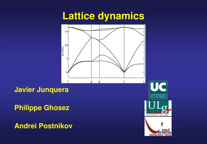
Lattice dynamics. Javier Junquera. Philippe Ghosez. Andrei Postnikov. Warm up: a little bit of notation. Greek characters ( ) refer to atoms within the unit cell Latin characters ( ) refer to the different replicas of the unit cell . Position of atom in unit cell .

E N D
Lattice dynamics Javier Junquera Philippe Ghosez Andrei Postnikov
Warm up: a little bit of notation Greek characters ( ) refer to atoms within the unit cell Latin characters ( ) refer to the different replicas of the unit cell Position of atom in unit cell Vector defining the position of unit cell Position of atom within the unit cell Assuming periodic boundary conditions
…but the ions do not sit without moving; they oscillate around the mean equilibrium positions Here we shall assume that the instantaneous position of atom in unit cell will deviate from its mean equilibrium position by a small deviation , and we may write at any given time We shall assume that the typical excursions of each ion from its equilibrium position are small compared with the interionic spacing
Total energy of a periodic crystal with small lattice distortions We shall remain in the adiabatic approximation, in which it is considered that the electrons are in their ground state for any instantaneous ionic configuration Some considerations 1. In principle, if we take all the orders in the expansion (see the dot, dot, dot at the right), this expression is exact. 2. All the derivatives are taken at the mean equilibrium positions. They are constants in the expansion. 3. Since, the derivatives are taken at the equilibrium positions, the first derivatives in the previous expansion vanish.
Total energy of a periodic crystal with small lattice distortions in the harmonic approximation We shall now consider ionic displacements that are small compared with the interatomic spacing. Then, we can consider that all the terms beyond the quadratic one are negligible (a small number to the cube is much smaller than a small number to the square). This approximation is called the harmonic approximation The total energy of a periodic crystal in the harmonic approximation can be written
Interatomic force constants in real space: definitions and symmetry properties Translation invariance upon displacement of the lattice by an arbitrary lattice constant: the second derivative of the energy can only depend on the difference between and The second derivatives of the energy, coupling constants, are defined as the interatomic force constants in real space They must satisfy a number of conditions that arise from Isotropy of space Point group symmetry
The classical equation of motion for the ions Force exerted on atom in unit cell by all the other ions and the electronic cloud Acceleration of atom in unit cell By definition of force By definition of acceleration In cartesian components In cartesian components
The classical equation of motion for the ions For each atom, there are three equations of motion of this type (one for each cartesian direction). In total, Since Then
The classical equation of motion for the ions: a system of coupled equations We require the displacement of atom , in unit cell , along cartesian direction , To know the displacement of atom , in unit cell , along cartesian direction , For each atom, there are three equations of motion of this type (one for each cartesian direction). In total, The equations of motion are coupled
The classical equation of motion for the ions: seeking for a general solution (temporal dependency) We seek for general solutions where all the displacements have a temporal dependency of the form For each atom, there are three equations of motion of this type (one for each cartesian direction). In total, :index for the different solutions to the equations (index of mode) The equations of motion are coupled First ansatz: temporal dependency
The classical equation of motion for the ions: seeking for a general solution (spatial dependency) For each atom, there are three equations of motion of this type (one for each cartesian direction). In total, The equations of motion are coupled Second ansatz: spatial dependency For periodic structures, we can write the displacements in terms of a plane wave with respect to cell coordinates In contrast to a normal plane wave, this wave is only defined at the lattice point
A few properties and consequences of the ansatz is the component along direction of a vector called the polarization vector of the normal mode For periodic structures, we can write the displacements in terms of a plane wave with respect to cell coordinates The vibration of the ions have been classified according to a wave vector - Approach equivalent to that taken for the electrons through the Bloch theorem - If the solid is simulated by a supercell composed of N unit cells + Born-von Karman boundary conditions, then only compatible points can be used in the previous expression. There are as many allowed values as unit cells there are in the supercell In contrast to a normal plane wave, this wave is only defined at the lattice points
A little bit of algebra in the equation of motion: taking the time derivatives of the ansatz equation Now we replace the ansatz solution in the equation of motion Remember that the ansatz is Taking the time derivatives
A little bit of algebra in the equation of motion: replacing the ansatz in the equation Multiplying both sides by Reordering the sums, and multiplying both sides by
A little bit of algebra in the equation of motion: introducing the interatomic force constant The summation in must be performed over all the unit cells. Since the interatomic force constants in real space depend only on the relative distance between the atoms, the origin does not play a role anymore, and can be set to 0. Definition of the interatomic force constant in real space Then, the previous equation takes the form
A little bit of algebra in the equation of motion: the Fourier transform of the interatomic force constant The term in brackets is nothing else than the discrete Fourier transform of the interatomic force constant in real space Therefore, the movement of the atoms can be defined in terms of the following dynamical equations
The equation of motion in matricial form For each vector, we have a linear homogenous system of equations, that in matrix form can be read as Fourier transform of the interatomic force constants Mass matrix Phonon eigendisplacements Phonon frequencies Phonon eigendisplacements
The mass matrix: example for a system with two atoms in the unit cell Atom 1 Direction x Atom 1 Direction y Atom 1 Direction z Atom 2 Direction x Atom 2 Direction y Atom 2 Direction z Atom 1 Direction x Atom 1 Direction y Atom 1 Direction z Atom 2 Direction x Atom 2 Direction y Atom 2 Direction z
A renormalization of the displacements by the square root of the mass allows to solve a standard eigenvalue problem This is not a standard eigenvalue problem due to the presence of the mass matrix (somehow the “eigenvalue” changes from one row to the other…) We can recover an standard eigenvalue problem redefining the eigenvectors incorporating the square root of mass
The dynamical equation with the renormalized displacements Redoing previous algebra We define the dynamical matrix as So finally the dynamical equation reduces to
The dynamical equation with the renormalized displacements Redoing previous algebra In matrix form Dynamical matrix Phonon eigenvectors Phonon frequencies Phonon eigenvectors
The dynamical matrix is Hermitian By definition The transpose of the dynamical matrix is … …and the complex conjugate of the transpose
Relation between phonon eigenvectors and phonon eigendisplacements In a standard code, the dynamical matrix is diagonalized, and the solutions are the phonon eigenvectors However, to compute many properties related with the lattice dynamics, we require the phonon eigendisplacements. For instance, the mode polarity Required to compute, for instance, the static dielectric constant The phonon eigendisplacements and phonon eigenvectors are related by
Normalization of the phonon eigenvectors and phonon eigendisplacements For the phonon eigenvectors, at a given m and For the phonon eigendisplacements, at a given m and
How to compute the force constant matrix in reciprocal space: perturbation theory By definition Combining density functional with first-order perturbation theory: Density Functional Perturbation Theory (DFPT) Advantages: Disadvantages: It allows to keep the simplicity of a single cell calculation, whatever q-vector which is considered, and that can even be incommensurate with the crystal lattice Requires some additional implementation effort
How to compute the force constant matrix in real space: finite displacement technique …we can compute the dynamical matrix for every q-point Knowing the force constant matrix in real space… By definition We displace the atom in the unit cell along direction , and compute how changes the force on atom in unit cell along direction The derivative is computed by finite differences
How to compute the force constant matrix in real space: finite displacement technique …we can compute the dynamical matrix for every q-point Knowing the force constant matrix in real space… By definition In principle, we should displace the atoms in the unit cell one by one in all the three cartesian directions, and look at the force on the atom of our choice, that might be in a unit cell very far away. From a practical point of view, the values of the force constant matrix in real space decay with the distance between the atoms… so, practically the previous sum is cut to include only a given number of distant neighbours
How to compute phonons in Siesta: Use of the Vibra suite. Step 1: Build the supercell Unit cell in real space Supercell in real space
How to compute phonons in Siesta: Use of the Vibra suite. Step 1: Build the supercell We prepare an input file to run fcbuild and generate the supercell. Let´s call this input file Si.fcbuild.fdf Variables to define the unit cell in real space Variables to define the supercell in real space
How to compute phonons in Siesta: Use of the Vibra suite. Step 1: Build the supercell $siesta/Utils/Vibra/Src/fcbuild < Si.fcbuild.fdf • This will generate a file called FC.fdf with: • The structural data of the supercell (supercell lattice vectors, atomic coordinates,…) • The atoms that will be displaced to compute the interatomic force constants in real space • The amount that the atoms will be displaced The supercell should contain enough atoms so that all non-neglegeable elements of the force constant matrix are computed. The range in real space in which the force constant matrix decays to zero varies widely from system to system!!.
How to compute phonons in Siesta: Use of the Vibra suite. Step 2: Displace the atoms in the unit cell and compute IFC Unit cell in real space Supercell in real space Ideally, we should displace only the atoms in the unit cell, but this is not possible when using periodic boundary conditions… again, it is important to converge the size of the supercell
How to compute phonons in Siesta: Use of the Vibra suite. Step 2: Displace the atoms in the unit cell and compute IFC We prepare an input file to run siesta and compute the interatomic force constant matrix. Let´s call this input file Si.ifc.fdf Many variables are taken directly from the file where the supercell is described Only the atoms of the unit cell are displaced
How to compute phonons in Siesta: Use of the Vibra suite. Step 2: Displace the atoms in the unit cell and compute IFC $siesta/Obj/siesta < Si.ifc.fdf > Si.ifc.out This will generate a file called SystemLabel.FC with the interatomic force constant matrix Displace atom 1 along direction -x As many lines as atoms in the supercell, force on the atom j in the supercell (in eV/Å) Then loop on the directions along which the atom 1 is displaced: -x, +x, -y, +y, -z, +z Finally, loop on the atoms in the unit cell
How to compute phonons in Siesta: Use of the Vibra suite. Step 3: Compute the dynamical matrix and diagonalize Once the interatomic force constant matrix has been computed, a Fourier transform is carried out at different k-points to calculate the dynamical matrix The k-points are defined in the same way as to compute the electronic band structure in the same file used to define the supercell (Si.fcbuild.fdf)
How to compute phonons in Siesta: Use of the Vibra suite. Step 3: Compute the dynamical matrix and diagonalize $siesta/Utils/Vibra/Src/vibrator < Si.fcbuild.fdf Output: SystemLabel.bands: mode frequencies (in cm-1) (Same structure as the electronic band structure) SystemLabel.vectors: eigenmodes for each k-point (format self-explained) To plot the phonon band structure: $bandline.x < Si.bands > Si.bands.dat $gnuplot $plot “Si.bands.dat” using 1:2 with lines
Convergence of the phonon structure with the size of the supercell 1 1 1 2 2 2 3 3 3 Plane waves + pseudopotentials Dots represent experimental points P. E. Van Camp et al., Phys. Rev. B 31, 4089 (1985)