Download
1 / 64
680 likes | 1.02k Views
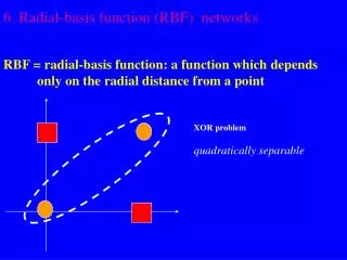
NEURAL NETWORK Radial Basis Function. RBF. Radial Basis Functions. The RBF networks, just like MLP networks, can therefore be used classification and/or function approximation problems.

E N D
Radial Basis Functions • The RBF networks, just like MLP networks, can therefore be used classification and/or function approximation problems. • The RBFs, which have a similar architecture to that of MLPs, however, achieve this goal using a different strategy: ……….. Linear output layer Input layer Nonlinear transformation layer (generates local receptive fields)
Radial Basis Function A hidden layer of radial kernels The hidden layer performs a non-linear transformation of input space The resulting hidden space is typically of higher dimensionality than the input space An output layer of linear neurons The output layer performs linear regression to predict the desired targets Dimension of hidden layer is much larger than that of input layer Cover’s theorem on the separability of patterns “A complex pattern-classification problem cast in a high-dimensional space non-linearly is more likely to be linearly separable than in a low-dimensional space” Support Vector Machines. RBFs are one of the kernel functions most commonly used.
Radial Basis Function j ( X ) 1 X w 1 m j x1 i å ( X ) = j y w ( X ) 2 w i i 2 = i 1 Output x2 å w 3 y j ( X ) x3 3 w ... m 1 ... More likely to be linearly separated x N j ( X ) m 1 Increased dimension: j ( X ) : non linear function N->m1 i RBFs have their origins in techniques for performing exact function interpolation [Bishop, 1995]
ARCHITECTURE • Input layer: source of nodes that connect the NN with its • environment. x1 w1 x2 y wm1 xm • Hidden layer: applies a non-linear transformation from the input space to the hidden space. • Output layer: applies a linear transformation from the hidden space to the output space.
φ-separability of patterns Hidden function Hidden space A (binary) partition, also called dichotomy, (C1,C2) of the training set C is φ-separable if there is a vector w of dimension m1 such that:
Examples of φ-separability Separating surface: Examples of separable partitions (C1,C2): Linearly separable: Quadratically separable: Polynomial type functions Spherically separable:
x1 x2 xm HIDDEN NEURON MODEL • Hidden units: use a radial basis function the output depends on the distance of the input x from the center t φ( || x - t||2) φ( || x - t||2) t is called center is called spread center and spread are parameters
Hidden Neurons • A hidden neuron is more sensitive to data points near its center. This sensitivity may be tuned by adjusting the spread . • Larger spread less sensitivity
φ : center Small Large Gaussian Radial Basis Function φ is a measure of how spread the curve is:
Types of φ • Multiquadrics: • Inverse multiquadrics: • Gaussian functions:
Nonlinear Receptive Fields • The hallmark of RBF networks is their use of nonlinear receptive fields • RBFs are universal approximators ! • The receptive fields nonlinearly transforms (maps) the input feature space, where the input patterns are not linearly separable, to the hidden unit space, where the mapped inputs may be linearly separable. • The hidden unit space often needs to be of a higher dimensionality • Cover’s Theorem (1965) on the separability of patterns: A complex pattern classification problem that is nonlinearly separable in a low dimensional space, is more likely to be linearly separable in a high dimensional space.
x2 (0,1) (1,1) 0 1 y x1 (0,0) (1,0) Example: the XOR problem • Input space: • Output space: • Construct an RBF pattern classifier such that: • (0,0) and (1,1) are mapped to 0, class C1 • (1,0) and (0,1) are mapped to 1, class C2
φ2 (0,0) Decision boundary 1.0 0.5 (1,1) 1.0 φ1 0.5 (0,1) and (1,0) Example: the XOR problem • In the feature (hidden) space: • When mapped into the feature space < 1 , 2 >, C1 and C2become linearly separable. Soa linear classifier with 1(x) and 2(x) as inputs can be used to solve the XOR problem.
(1,1) _ _ _ _ _ _ 1.0 0.8 0.6 0.4 0.2 0 (0,1) (1,0) (0,0) | | | | | | 0 0.2 0.4 0.6 0.8 1.0 1.2 The (you guessed it right) XOR Problem Consider the nonlinear functions to map the input vector x to the 1- 2 space x2 1 x=[x1 x2] 0 x1 0 1 The nonlinear function transformed a nonlinearly separable problem into a linearly separable one !!!
Initial Assessment • Using nonlinear functions, we can convert a nonlinearly separable problem into a linearly separable one. • From a function approximation perspective, this is equivalent to implementing a complex function (corresponding to the nonlinearly separable decision boundary) using simple functions (corresponding to the linearly separable decision boundary) • Implementing this procedure using a network architecture, yields the RBF networks, if the nonlinear mapping functions are radial basis functions. • Radial Basis Functions: • Radial: Symmetric around its center • Basis Functions: A set of functions whose linear combination can generate an arbitrary function in a given function space.
x1 uJi xd RBF Networks d inputnodes H hidden layer RBFs(receptive fields) x1 c outputnodes 1 z1 x2 ……... .. Wkj netk Uji zk …….... j .. yj Linear act. function zc … x(d-1) H xd : spread constant
x1 UJi xd Principle of Operation Euclidean Norm : spread constant yJ y1 wKj yH Unknowns: uji, wkj,
Principle of Operation • What do these parameters represent? • Physical meanings: • : The radial basis function for the hidden layer. This is a simple nonlinear mapping function (typically Gaussian) that transforms the d- dimensional input patterns to a (typically higher) H-dimensional space. The complex decision boundary will be constructed from linear combinations (weighted sums) of these simple building blocks. • uji: The weights joining the first to hidden layer. These weights constitute the center points of the radial basis functions. • : The spread constant(s). These values determine the spread (extend) of each radial basis function. • Wjk: The weights joining hidden and output layers. These are the weights which are used in obtaining the linear combination of the radial basis functions. They determine the relative amplitudes of the RBFs when they are combined to form the complex function.
Principle of Operation wJ:Relative weight of Jth RBF J: Jth RBF function J * uJCenter of Jth RBF
Learning Algorithms • Parameters to be learnt are: • centers • spreads • weights • Different learning algorithms
Learning Algorithm 1 • Centers are selected at random • center locations are chosen randomly from the training set • Spreads are chosen by normalization:
Learning Algorithm 1 • Weights are found by means of pseudo-inverse method Desired response Pseudo-inverse of
Learning Algorithm 2 • Hybrid Learning Process: • Self-organized learning stage for finding the centers • Spreads chosen by normalization • Supervised learning stage for finding the weights, using LMS algorithm • Centers are obtained from unsupervised learning (clustering). • Spreads are obtained as variances of clusters, w are obtained through LMS algorithm. Clustering (k-means) and LMS are iterative. This is the most commonly used procedure. Typically provides good results.
Learning Algorithm 2: Centers • K-means clustering algorithm for centers • Initialization: tk(0) random k = 1, …, m1 • Sampling: draw x from input space C • Similaritymatching: find index of best center • Updating: adjust centers • Continuation: increment n by 1, goto 2 and continue until no noticeable changes of centers occur
Learning Algorithm 3 • Supervised learning of all the parameters using the gradient descent method • Modify centers • All unknowns are obtained from supervised learning. Instantaneous error function Learning rate for Depending on the specific function can be computed using the chain rule of calculus
Learning Algorithm 3 • Modify spreads • Modify output weights
RBFs Training [Haykin, 1999] Unsupervised selection of RBF centers RBF centers are selected so as to match the distribution of training examples in the input feature space Supervised computation of output vectors Hidden-to-output weight vectors are determined so as to minimize the sum squared error between the RBF outputs and the desired targets Since the outputs are linear, the optimal weights can be computed using fast, linear matrix inversion Once the RBF centers have been selected, hidden-to-output weights are computed so as to minimize the MSE error at the output
Polynomial model family Linear inwReduces to the linear regression case, but with more variables. Number of terms grows asDM
Generalized linear model Linear inwReduces to the linear regression case, but with more variables. Requires good guess on “basis functions”hk(x)
Polynomial Classifier: XOR problem • XOR problem with polynomial function. • With nonlinear polynomial functions classes can be classified. • Example XOR-Problem: …but with a polynomial function!
Polynomial Classifier more general
The Gaussian is the most commonly used RBF • Note that • Gaussian RBFs are localized functions ! unlike the sigmoids used by MLPs Using sigmoidal radial basis functions Using Gaussian radial basis functions
1. Function Width Demo • Application Model • Function Approximation • Target Function • Focus • The width and the center of RBF. • Generalization of RBF Network
Change the width of RBF (1) • Radial Basis Function model : Gaussian • Test Case • The number of RBF(neuron) is fixed : 21 • Case 1: width = 1 • Case 2: width = 0.2 • Case 3: width = 200 • Validation Test • To check the generalization ability of RBF Networks
Change the width of RBF (2) Width = 1 Width = 0.2 Width = 200
Change the number of RBF center (1) • Test Case • The Number of RBF = 7 center position: [-8, –5, –2, 0, 2, 5, 8] • Case 1: width = 1 • Case 2: width = 6 • The Number of RBF = 2 center position: [-3, 10] • Case 3: width = 1 • Case 4: width = 6
Change the number of RBF center (2) • # of RBF = 7 [-8, -5, -2, 0, 2, 5, 8] width = 1 width = 6
Change the number of RBF center (3) • # of RBF = 2 [ -3, 10] width = 1 width = 6