Download
1 / 122
1.22k likes | 1.22k Views
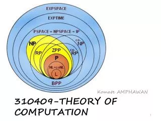
::ICS 804:: Theory of Computation - Ibrahim Otieno - iotieno@uonbi.ac.ke +254-0722-429297 SCI/ICT Building Rm. 214. Course Outline. Mathematical Preliminaries Turing Machines Recursion Theory Markov Algorithms Register Machines Regular Languages and finite-state automata

E N D
::ICS 804:: Theory of Computation - Ibrahim Otieno - iotieno@uonbi.ac.ke +254-0722-429297 SCI/ICT Building Rm. 214
Course Outline • Mathematical Preliminaries • Turing Machines • Recursion Theory • Markov Algorithms • Register Machines • Regular Languages and finite-state automata • Aspects of Computability
Last Week: Discrete Mathematics • Topics: • Set-theoretic concepts • Formal language theory • Functions • Big-O notation • Propositional logic • Proof Techniques • Number-theoretic predicates
Course Outline • Mathematical Preliminaries • Turing Machines • Recursion Theory • Markov Algorithms • Register Machines • Regular Languages and finite-state automata • Aspects of Computability
Turing Machines • What is Computation? • Informal Description of Turing Machines • Formal Description of Turing Machines • Turing Machines as Language acceptors and Language recognizers • Turing Machines as Computers of number-theoretic functions • Modular Turing Machines • Complexity Theory
Computation • Think of machines: Computers and calculators • Until 1930s: computation done solely by human beings • Computation is a cultural phenomenon • Most typical example: numeric computation • 34239 + 23478378 • 2347 - 293874 • 43.3421 • 3.24 • 72% of the population of Nairobi
Computation • But also: non-numeric computation (operations on strings of symbols) • Sorting a set of strings • alphabetizing • Find the length of string ababababbbaba • What is abababbabbabR? • Is abababbbbbababa a palindrome? • What is the longest substring common to GCATCCTAA and ATACTAATCCTTA?
Algorithm • Related to the concept of an algorithm • Informal definition of algorithm: • a certain sort of general method for solving a family of related questions e.g. truth table algorithm for argument validity in propositional calculus • End result of the mathematician’s quest for a general procedure for answering any one of some infinitefamily of questions
Algorithm - example Question template: is natural number n a prime number? Corresponds to an infinite family of yes/no questions: is natural number 1 a prime number? is natural number 2 a prime number? is natural number 3 a prime number? …
Algorithm - example Question template: is natural number n a prime number? Decision problem is natural number 1 a prime number? is natural number 2 a prime number? is natural number 3 a prime number? … Instance of the general problem
Algorithm - example What if n is large, e.g. 807 or 907 • Attempt successive division by divisors k=2,3,4,… up to a certain point • If k is seen to divide n without a remainder, it is not a prime number
Algorithm - example What if n is large, e.g. 807 or 907 • Attempt successive division by divisors k=2,3,4,… up to a certain point • If k is seen to divide n without a remainder, it is not a prime number
Algorithm • This algorithm may involve many steps, but is always determinate • Always gives a definite answer • Decision problem expressed by question template is natural number n a prime number? is a decidable problem
Algorithm What-questions ( yes/no questions) What is the nth prime number? Algorithm for Finding the nth Prime Number Input: natural number n 1 Output: the nth prime number Begin i := 1; k := 1; while i n do begin k := k + 1; if k is prime then i := i+1 end; return k end.
Algorithms • Procedure to answer an infinite number of questions • Algorithm itself must be finitely described • Definite: at each step there is a determinate next step (“mechanical”): deterministic • Finite process: finite number of steps to solve the problem • Conclusive: when the algorithm terminates an unambiguous result or “output” must be generated
Three Computational Paradigms • Number-theoretic function computation (functions from N to N) • Language acceptance (recognition) • Transduction (transformation of an input into an appropriate output) • Turing machines implement each of these paradigms
Three Computational Paradigms • Number-theoretic function computation (functions from N to N) • Language acceptance (recognition) • Transduction (transformation of an input into an appropriate output)
Number-theoretic Functions (recap) • Number-theoretic functions: map natural numbers unto natural numbers • Unary number-theoretic functions f(n) = n + 1 Binary number-theoretic functions f: N2N f(n,m) = n + m • K-ary number-theoretic functions f: NkN • 0-ary number theoretic functions C02: N0N C02() = 2
Number-theoretic functions • Computation of a given k-ary number-theoretic function f • Computation of the unique value f(n1,n2,…,nk) of n given arguments n1,n2,…,nk
Number-theoretic functions • Computable function: no definition, but describe what it means for a number-theoretic function to be computable
Number-theoretic functions • Example: f(n) = the nth primary number f(1) = 2 f(2) = 3 f(3) = 5 … • Computation involved for f(1000) • Computable: given any natural number n one can find the value of f for argument n (using the algorithm defined earlier)
Number-theoretic functions • Binary function g(n,m) = n / m • Effectively calculable: we possess an algorithm that produces after a finite number of steps, the correct value of g for any argument pair <n,m> • Effectiveness of g • Partial function (undefined for <n,0>): g’s partiality does not compromise its effectiveness • If g(n,m) is undefined the algorithm should not return a value
Function Computation Paradigm • Computing the value of a numeric function is a paradigmatic instance of the phenomenon we call computation • Function computation paradigm • Also other types of computation, not involving function computation
Three Computational Paradigms • Number-theoretic function computation (functions from N to N) • Language acceptance (recognition) • Transduction (transformation of an input into an appropriate output)
Language Recognition Paradigm Finite string w from * with = {a,b} abbbabababbbabbbabababbba Determine whether w is palindrome
Language Recognition Paradigm • Finite string w from * with = {a,b} abbbabababbbabbbabababbba • Determine whether w is palindrome If leftmost and rightmost symbol are identical, remove them. Iterate until (1) leftmost remaining symbol is not identical with rightmost remaining symbol (2) just one symbol remains (3) no symbol remains • (2,3): w is a palindrome • (1): w is not a palindrome
Language Recognition Paradigm • No numerical computation involved! • Only symbol manipulation (removing, comparing, … symbols) Does w (abbbabababbbabbbabababbba) contain the same number of a’s and b’s? • Remove leftmost occurrence of a together with leftmost occurrence of b until (1) no symbols remain (2) just a’s remain (3) just b’s remain (1): na(w) = nb(w) (2,3): na(w) nb(w)
Language Recognition Paradigm • Compute whether or not the original string belongs to the class of strings possessing a certain property (e.g. palindromes) • String classification paradigm • Language recognition paradigm
Formal Language (recap) • * set of all words over • Language over : any subset of * • Empty language: • Universal language: * • Unit language L = {w}
Language Recognition Paradigm • Determine whether or not an arbitrary word w belongs to some language L where L is assumed to be given/defined in advance. • An algorithm that successfully does this in the case of language L will be said to recognize L • Redefine into language recognition problem: LPrime = {11,111,11111,1111111,…}
Three Computational Paradigms • Number-theoretic function computation (functions from N to N) • Language acceptance (recognition) • Transduction (transformation of an input into an appropriate output)
Transduction paradigm • Computation that involves some well-defined transformation (transduction) of symbol strings e.g. reversing a word w = aabaabb and wR = bbaabaa
Paradigms • Study computability: • Function computation paradigm: in-principle computability • Language/recognition: when we need to take time/space resources into account • But: paradigm inter-reducibility: so no real emphasis necessary • Language function: translate symbols into numeric values (e.g. ASCII codes)
Representing Natural Numbers • Unary notation • 111 represents natural number 2 • The “extra” 1 is the representational 1 • Why do we need the representational 1?
Representing Natural Numbers • Unary notation • 111 represents natural number 2 • The “extra” 1 is the representational 1 • Why do we need the representational 1? we need to be able to represent 0
Models of Computation • Try to characterize/analyze the intuitive notion of computable function • Effectively calculable function: addition, word reversal, …: part of cultural heritage: • It is pretheoretic • Non-mathematical, philosophical concept • !!!! Models of computable function (turing-computable function, …): technical concepts as opposed to computable function
Models of Computation • Most famous model: Turing model • “On Computable Numbers, with an Application to the Entscheidungsproblem” (1936-1937) • Still the only frequently cited model outside computer science: standard for sequential computation
Feasible Computation • Computability in principle: computation in the absence of any restriction on either time or space • Computational feasibility • A computation is feasible if it would consume only a quantity of resources that does not exceed what is likely to be available to the computational process e.g. is n prime? Algorithm that requires n division steps: feasible since each step involves a reasonable number of computation steps • Intuition of feasibility ( economically cost-effective, …) • Infeasibility = not cost-effective • Feasibility is a philosophical concept
Example • State diagram (transition diagram): full description of machine M’s behavior • Machine states and instructions • Initial state q0 • Machine instructions
Example • Read/write (tape) tape (tape squares) • B: blank tape square • Read/write head scans one tape square • Initial tape configuration
M initially B • Machine configuration: In state q0 scanning a blank tape square
M after One Computation Step • Machine configuration: In state q1 scanning an a (all other squares blank).
M after 2 Computation Steps • Machine configuration: In state q2
M after 3 Computation Steps b • Machine configuration: In state q3
M after 4 Computation Steps b • Machine configuration: In state q4
Summary of M’s Behavior • When started scanning squares on a completely blank tape, M writes ab and halts scanning a. • We makes no claims for M if tape not initially blank.
Important Concepts • Tape configuration: content of M’s tape + location of M’s read/write head on it at any given step in M’s computation • Machine configuration = tape configuration + current state e.g. final machine configuration: M is in state q4 with its tape configured as b