Download
1 / 55
570 likes | 746 Views
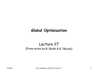
Global Optimization. Lecture 22. Lecture Outline. Global flow analysis Global constant propagation Liveness analysis. X := 3 Y := Z * W Q := 3 + Y. Y := Z * W Q := 3 + Y. Local Optimization. Recall the simple basic-block optimizations Constant propagation Dead code elimination.

E N D
Global Optimization Lecture 22 Prof. Fateman CS 164 Lecture 22
Lecture Outline • Global flow analysis • Global constant propagation • Liveness analysis Prof. Fateman CS 164 Lecture 22
X := 3 Y := Z * W Q := 3 + Y Y := Z * W Q := 3 + Y Local Optimization Recall the simple basic-block optimizations • Constant propagation • Dead code elimination X := 3 Y := Z * W Q := X + Y Prof. Fateman CS 164 Lecture 22
Global Optimization These optimizations can be extended to an entire control-flow graph X := 3 B > 0 Y := Z + W Y := 0 A := 2 * X Prof. Fateman CS 164 Lecture 22
Global Optimization These optimizations can be extended to an entire control-flow graph X := 3 B > 0 Y := Z + W Y := 0 A := 2 * X Prof. Fateman CS 164 Lecture 22
Global Optimization These optimizations can be extended to an entire control-flow graph X := 3 B > 0 Y := Z + W Y := 0 A := 2 * 3 Prof. Fateman CS 164 Lecture 22
X := 3 B > 0 Y := Z + W X := 4 Y := 0 A := 2 * X Correctness • How do we know it is OK to globally propagate constants? • There are situations where it is incorrect: Prof. Fateman CS 164 Lecture 22
Correctness (Cont.) To replace a use of x by a constant k we must know that: On every path to the use of x, the last assignment to x is x := k ** Prof. Fateman CS 164 Lecture 22
Example 1 Revisited X := 3 B > 0 Y := Z + W Y := 0 A := 2 * X Prof. Fateman CS 164 Lecture 22
X := 3 B > 0 Y := Z + W X := 4 Y := 0 A := 2 * X Example 2 Revisited Prof. Fateman CS 164 Lecture 22
Discussion • The correctness condition is not trivial to check • “All paths” includes paths around loops and through branches of conditionals • Checking the condition requires global analysis • An analysis of the entire control-flow graph Prof. Fateman CS 164 Lecture 22
Global Analysis Global optimization tasks share several traits: • The optimization depends on knowing a property X at a particular point in program execution • Proving X at any point requires knowledge of the entire function body • It is OK to be conservative. If the optimization requires X to be true, then want to know either • X is definitely true • Don’t know if X is true • It is always safe to say “don’t know” Prof. Fateman CS 164 Lecture 22
Global Analysis (Cont.) • Global dataflow analysis is a standard technique for solving problems with these characteristics • Global constant propagation is one example of an optimization that requires global dataflow analysis Prof. Fateman CS 164 Lecture 22
Global Constant Propagation • Global constant propagation can be performed at any point where ** holds • Consider the case of computing ** for a single variable X at all program points Prof. Fateman CS 164 Lecture 22
Global Constant Propagation (Cont.) • To make the problem precise, we associate one of the following values with X at every program point Prof. Fateman CS 164 Lecture 22
X = * X = 3 X = 3 X = 3 X = * X = * X := 3 B > 0 X = 4 X = 3 X = 3 Y := Z + W X := 4 Y := 0 A := 2 * X Example Prof. Fateman CS 164 Lecture 22
Using the Information • Given global constant information, it is easy to perform the optimization • Simply inspect the x = ? associated with a statement using x • If x is constant at that point replace that use of x by the constant • But how do we compute the properties x = ? Prof. Fateman CS 164 Lecture 22
The Idea The analysis of a complicated program can be expressed as a combination of simple rules relating the change in information between adjacent statements Prof. Fateman CS 164 Lecture 22
Explanation • The idea is to “push” or “transfer” information from one statement to the next • For each statement s, we compute information about the value of x immediately before and after s Cin(x,s) = value of x before s Cout(x,s) = value of x after s Prof. Fateman CS 164 Lecture 22
Transfer Functions • Define a transfer function that transfers information one statement to another • In the following rules, let statement s have immediate predecessor statements p1,…,pn Prof. Fateman CS 164 Lecture 22
X = * Rule 1 (unknown predecessor) if Cout(x, pi) = * for any predecessor i, then Cin(x, s) = * X = * X = ? X = ? X = ? s Prof. Fateman CS 164 Lecture 22
X = * Rule 2 (different predecessors) If Cout(x, pi) = c and Cout(x, pj) = d and d <> c then Cin (x, s) = * X = d X = ? X = c X = ? s Prof. Fateman CS 164 Lecture 22
X = c Rule 3 (exclude unreachable values) if Cout(x, pi) = c or # for all i, then Cin(x, s) = c X = c X = # X = c X = # s Prof. Fateman CS 164 Lecture 22
Rule 4 (unreachable propagation) if Cout(x, pi) =# for all i, then Cin(x, s) = # X = # X = # X = # X = # X = # s Prof. Fateman CS 164 Lecture 22
The Other Half • Rules 1-4 relate the out of one or more statements to the in of the successor statement • Now we need rules relating the in of a statement to the out of the same statement Prof. Fateman CS 164 Lecture 22
X = # X = # Rule 5 Cout(x, s) =# if Cin(x, s) = # s Prof. Fateman CS 164 Lecture 22
X = ? X = c Rule 6 Cout(x, x := c) =c if c is a constant x := c Prof. Fateman CS 164 Lecture 22
X = ? X = * Rule 7 Cout(x, x := f(…)) =* x := f(…) Prof. Fateman CS 164 Lecture 22
X = a X = a Rule 8 Cout(x, y := …) =Cin(x, y := …) if x <> y y := . . . Prof. Fateman CS 164 Lecture 22
An Algorithm • For every entry s to the program, set Cin(x, s) = * • Set Cin(x, s) = Cout(x, s) = # everywhere else • Repeat until all points satisfy 1-8: Pick s not satisfying 1-8 and update using the appropriate rule Prof. Fateman CS 164 Lecture 22
X = * X = 3 X = 3 X = 3 X = 3 The Value # • To understand why we need #, look at a loop X := 3 B > 0 Y := Z + W Y := 0 A := 2 * X A < B Prof. Fateman CS 164 Lecture 22
Discussion • Consider the statement Y := 0 • To compute whether X is constant at this point, we need to know whether X is constant at the two predecessors • X := 3 • A := 2 * X • But info for A := 2 * X depends on its predecessors, including Y := 0! Prof. Fateman CS 164 Lecture 22
The Value # (Cont.) • Because of cycles, all points must have values at all times • Intuitively, assigning some initial value allows the analysis to break cycles • The initial value # means “So far as we know, control never reaches this point” Prof. Fateman CS 164 Lecture 22
X = * X = 3 X = 3 X = # X = # X = # X = 3 X = 3 Example X := 3 B > 0 Y := Z + W Y := 0 A := 2 * X A < B Prof. Fateman CS 164 Lecture 22
X = * X = 3 X = 3 X = # X = # X = 3 X = 3 X = 3 Example X := 3 B > 0 Y := Z + W Y := 0 A := 2 * X A < B Prof. Fateman CS 164 Lecture 22
X = * X = 3 X = 3 X = # X = 3 X = 3 X = 3 X = 3 Example X := 3 B > 0 Y := Z + W Y := 0 A := 2 * X A < B Prof. Fateman CS 164 Lecture 22
X = * X = 3 X = 3 X = 3 X = 3 X = 3 X = 3 X = 3 Example X := 3 B > 0 Y := Z + W Y := 0 A := 2 * X A < B Prof. Fateman CS 164 Lecture 22
Orderings • We can simplify the presentation of the analysis by ordering the values # < c < * • Drawing a picture with “lower” values drawn lower, we get * -1 0 1 # Prof. Fateman CS 164 Lecture 22
Orderings (Cont.) • * is the greatest value, # is the least • All constants are in between and incomparable • Let lub be the least-upper bound in this ordering • Rules 1-4 can be written using lub: Cin(x, s) = lub { Cout(x, p) | p is a predecessor of s } Prof. Fateman CS 164 Lecture 22
Termination • In general, simply saying “repeat until nothing changes” doesn’t guarantee that eventually nothing changes. • The use of lub explains why the algorithm terminates • Values start as # and only increase • # can change to a constant, and a constant to * • Thus, C_(x, s) can change at most twice Prof. Fateman CS 164 Lecture 22
Termination (Cont.) Thus the algorithm is linear in program size Number of steps = Number of C_(….) values computed * 2 = Number of program statements * 4 Prof. Fateman CS 164 Lecture 22
Liveness Analysis Once constants have been globally propagated, we would like to eliminate dead code After constant propagation, X := 3 is dead (assuming X not used elsewhere) X := 3 B > 0 Y := Z + W Y := 0 A := 2 * X Prof. Fateman CS 164 Lecture 22
Live and Dead • The first value of x is dead (never used) • The second value of x is live (may be used) • Liveness is an important concept X := 3 X := 4 Y := X Prof. Fateman CS 164 Lecture 22
Liveness A variable x is live at statement s if • There exists a statement s’ that uses x • There is a path from s to s’ • That path has no intervening assignment to x Prof. Fateman CS 164 Lecture 22
Global Dead Code Elimination • A statement x := … is dead code if x is dead after the assignment • Dead statements can be deleted from the program • But we need liveness information first . . . Prof. Fateman CS 164 Lecture 22
Computing Liveness • We can express liveness in terms of information transferred between adjacent statements, just as in copy propagation • Liveness is simpler than constant propagation, since it is a boolean property (true or false) Prof. Fateman CS 164 Lecture 22
X = true Liveness Rule 1 Lout(x, p) = Ú { Lin(x, s) | s a successor of p } p X = ? X = ? X = true X = ? Prof. Fateman CS 164 Lecture 22
X = true X = ? Liveness Rule 2 Lin(x, s) =true if s refers to x on the rhs …:= f(x) Prof. Fateman CS 164 Lecture 22
X = false X = ? Liveness Rule 3 Lin(x, x := e) =false if e does not refer to x x := e Prof. Fateman CS 164 Lecture 22
X = a X = a Liveness Rule 4 Lin(x, s) =Lout(x, s) if s does not refer to x s Prof. Fateman CS 164 Lecture 22