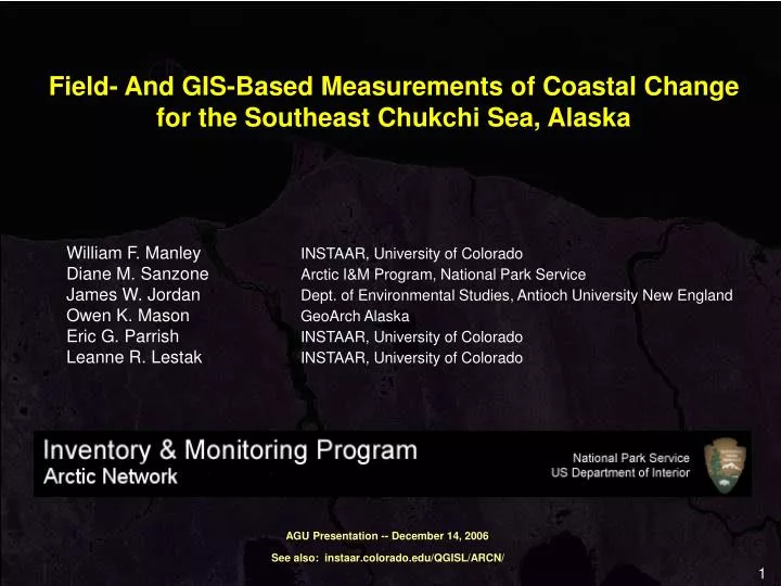
Field- And GIS-Based Measurements of Coastal Change for the Southeast Chukchi Sea, Alaska

1. Field- And GIS-Based Measurements of Coastal Change for the Southeast Chukchi Sea, Alaska William F. Manley INSTAAR, University of Colorado Diane M. Sanzone Arctic I&M Program, National Park Service James W. Jordan Dept. of Environmental Studies, Antioch University New England Owen K. Mason GeoArch Alaska Eric G. Parrish INSTAAR, University of Colorado Leanne R. Lestak INSTAAR, University of Colorado AGU Presentation -- December 14, 2006 See also: instaar.colorado.edu/QGISL/ARCN/

2. Coastal Erosion • Rapid, observable change to the environment • Multiple impacts on a variety of habitats • Fragile coast is a sensitive indicator of “stressors”: • direct human disturbance • climate change: • longer ice-free season • increased permafrost melting • change in frequency and intensity of storms • sea level rise

3. Goals • Field measurements as test of GIS approach • Preliminary GIS results

4. Study Area C h u k c h i S e a

5. Coastal Monitoring Stations • 27 sites • first established 1987-1994 • revisited in 2006 • measured on “bluff top”

6. Field Methods

7. Remote Sensing & GIS Approach • High-resolution base imagery 2003 • 2003 orthophoto mosaic • Historic aerial photographs ca. 1980 • orthorectified photos for ca. 1980 • orthorectified photos for ca. 1950 ca. 1950 • Comparison of different “time slices” allows us to detect and measure change • Imagery and data useful for other concerns

8. from NOAA & NPS 1:24,000 natural color photos • mosaic created by Aero-Metric • 0.6 m resolution • accuracy: 1.2 m (RMSE) • 112 tiles, 98 GB: lots of imagery! • highest res. in Alaska for this large of an area • available to the public early 2007 • valuable for other types of research

9. 60 frames Color IR 1.0 m res. • 57 frames • Color IR • 1:64,000 • 1.0 m resolution • 1.5 m accuracy (RMSE)

10. 130 frames Black & White 1.0 m res. • 108 frames • Black and White • 1:43,000 • 1.0 m resolution • 2.0 m accuracy (RMSE)

11. Shoreline Reference Feature (SRF):“bluff top” (wave-cut scarp) Barrier island or spit Mainland bluff Beach ridge complex

22. 2003

23. 1949

24. 1985

25. 2003

26. 1949

27. 1985

28. 2003

30. DSAS Thieler et al. (2005)

31. Baseline baseline

32. Transects

33. Transects 1949 1985 51.4 m ÷ 36 yr = 1.4 m/yr

34. “Early” Period ca. 1950 – ca. 1980m/yr 1949 1985

35. “Late” Period ca. 1980 – 2003m/yr 1985 2003

36. accretion

37. GIS Errors Shoreline Position (m) Coastal Change

38. r2 = 0.80 n = 21 1:1

39. mean difference: 0.12 m/yr r2 = 0.80 n = 21 1:1

40. GIS Errors Shoreline Position (m) Coastal Change Field Test (mean difference)

41. spatial variability • “early” erosion

42. accretion

43. station eroded • “late” erosion

44. “Early” Period ca. 1950 – ca. 1980 CAKR (n = 1628) BELA (n = 1146) xy plot

45. “Late” Period ca. 1980 – 2003 CAKR (n = 1628) BELA (n = 1146) xy plot

46. Is coastal erosion increasing with Arctic warming? xy plot

47. Conclusions • Field: • more precise • measurements more often • GIS: • acceptably low errors • comprehensive spatial analysis • Is global warming responsible?: • storm climatology important • high spatial and temporal resolution needed