Download
1 / 62
620 likes | 793 Views
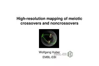
High-resolution mapping of meiotic crossovers and noncrossovers. Wolfgang Huber EMBL-EBI. Statistical and computational technology for the understanding of genotype - phenotype networks HT screening - RNAi, drugs, combinations Automated phenotyping from image analysis

E N D
High-resolution mapping of meioticcrossovers and noncrossovers Wolfgang Huber EMBL-EBI
Statistical and computational technology for the understanding of genotype - phenotype networks HT screening - RNAi, drugs, combinations Automated phenotyping from image analysis Genotyping from microarrays & new sequencing Machine learning & Data integration Bioconductor project
10 min: Visualisation of high density along genome data 35 min: Recombination
ChIP-Seq data and "pile-up" Solexa reads, aligned to genome "pile-up" vector Figure from Zhang et al., PLoS Comp. Biol. 2008
Pile-up plot for chromosome 10 H3K4me1 ChIP-Seq Barski et al. Cell 2007 H3K4me3
Zoom-in H3K4me1 H3K4me3
Hilbert plots of chromosome 10 H3K4me1 H3K4me3
History The concept of space-filling curves is due to Giuseppe Peano (1890). This specific curve has been invented by David Hilbert (1891). The idea to use these curves for visualization was first published by Daniel Keim (1996) for economics data.
3-colour Hilbert plot red: H3K4me1 green: H3K4me3 blue: exons
Availability Open source, released Oct 2008 under GPL v3 Bioconductor packages HilbertVis & HilbertVisGUI Stand-alone application: reads GFF and wiggle track files (incl. BED) Simon Anders
Meiotic recombination Proper chromosome segregation Increase of genetic diversity Gene A Gene B Gene C Gene A Gene b Gene c Gene a Gene b Gene c Gene a Gene B Gene C
Double-strand break repair CO: NCO: Recombination initiates with a double-strand break in one DNA molecule. Only two DNA molecules (homologs) are shown here. Slide18
Non-uniform distribution of recombination across the genome female average male Human chr. 22q Yeast chr. 3 Petes T.D., 2001 Baudat F. & Nicolas A., 1997 Recombination hotspots are small genomic regions where recombination events cluster, surrounded by stretches with little or no recombination activity.
Map all recombination events that occurred in 50 yeast meiosis using high-density tiling microarrays
Eugenio Mancera Ramos Richard Bourgon • Lars Steinmetz
Clinical isolates of S. cerevisiae Clinical strain (YJM789) Laboratory strain (S288c) The common lab yeast Isolated from rotten fig in California in 1930s Domesticated: related to baker's yeast, wine-making and beer-brewing yeasts Genome sequence of S288c: A Goffeau et al. Science (1996) Isolated from immuno-compromised patients Pathogenic in mouse model of systemic infection Various fungal pathogenic characteristics: pseudohyphae, colony morphology switching Ability to grow at >37˚C – a virulence trait Genome sequence of YJM789: W Wei et al., PNAS (2007): 60k SNPS, 6k indels wrt S288c
Experimental approach Mancera*, Bourgon*. Brozzi, Huber, Steinmetz (2008) Slide23
1 tiling array for 2 yeast genomes common S-specific Y-specific * 5’ 3’ Watson strand 8bp * 3’ 5’ Crick strand 4bp 25mer 10% 4% 86% S288c YJM789 291k 2,368k 108k Wei et al., PNAS (2007) Custom design manufactured by Affymetrix (probes)
Identification of previously unknown ncRNA and antisense transcripts and mapping of transcripts Antisense CBF1 David*, Huber* et al., (2006)
The computational & statistical challenges Genotyping marray probes and polymorphisms are in a many-to-many relationship Tiling array provides thorough coverage, but probes have variable performance wrt sensitivity & specificity (e.g. cross-hybridisation) We need highly accurate individual genotype calls if we want to detect small events Event rate inference Our data invert the traditional relationship between event and markers: instead of inferring crossovers between widely spaced markers, we have multiple markers over single events, both crossover and non-crossover Marker spacing influences detection rate, but in complicated ways Non-crossovers falling between markers are not observed Slide26
Genotyping “single feature polymorphisms” Hybridization efficiency depends on number and position of mismatches. Differential hybridization provides a means of detecting polymorphisms, even when only the reference genome sequence is known.Winzeler et al., Science 281(5380), 1998. Brem et al., Science 296(5568), 2002. Steinmetz et al., Nature 416(6878), 2002. Borevitz et al., Genome Research 13(3), 2003. Given parental behavior, segregants can be genotyped via supervised classification. Slide27
Tiling arrays, probe sets, markers Probe set: group of probes which each exactly map to a unique locus and which interrogate a common polymorphism. Marker: one or more polymorphisms interrogated by the same probe set. 6: CTTCACTATTTGTACAGATCGCAAT 5: CTAACTTCACTATTTGTACAGATCG 4: GGCCCTAACTTCACTATTTGTACAG 2: GACTGGCCCTAACTTCACTATTTGT 1: GGAGGACTGGCCCTAACTTCACTAT S96: CCTCCTGACCGGGATTGAAGTGATAAACATGTCTAGCGTTA YJM789: CCTCCTGACCGGGATTGAACTGATAAACATGTCTAGCGTTA 3: GACTGGCCCTAACTTGACTATTTGT
Multivariate probe set dataparallel coordinate plots Slide29
A multivariate method SNPScanner: Gresham et al., Science 311, 2006 Detailed parametric model of probe intensity xiwith and without presence of SNP as function of • Probe GC content • Position of SNP within the probe • Nucleotides surrounding the SNP Fit these model parameters using two sequenced strains with known SNPs To genotype a segregant or new strain at a given base, compute a Bayes factor assumption: covariance matrices diagonal and same
SNP Scanner ~ 97% correct calls – not enough for the reliable detection of conversion events Parental arrays are informative, but alone often do not predict segregant behaviour. Purely supervised classification (i) wastes information and (ii) may be misleading. Binary classification boundary is necessary but not sufficient. Shapes of class distributions (→confidence) are useful for QA/QC.
ssG: a semi-supervised, model-based genotyping algorithm 2-component Normal mixture model p(x) = 1 pN(x | m1, S1) + 2 pN(x | m2, S2) For each array i and each probeset: (Xi,Yi) with array data Xi and class variable Yi.Yi known for parental arrays, unknown for segregants. Fit with the EM algorithm.
ssG An instance of the EM algorithm applied to multivariate Gaussian mixture modeling: iteratively estimate class shapes and object class membership probabilities
ssG An instance of the EM algorithm applied to multivariate Gaussian mixture modeling: iteratively estimate class shapes and object class membership probabilities
ssG An instance of the EM algorithm applied to multivariate Gaussian mixture modeling: iteratively estimate class shapes and object class membership probabilities
Filtering ambiguous individual genotype calls Aberrant probe sets Weakly separating probesets Imbalanced probesets Probe Sets Genotype Calls
Recombination event inference for one tetrad median intermarker-distance: 78bp Slide43
Event size and marker resolution 4163 crossovers, 2126 non-crossovers across 46 meioses. Slide44
Inferring event rates Slide46
Recombination event rates Traditional corrections (e.g., Haldane) use recombination fraction, and adjust for unseen crossovers which occur between widely-spaced markers. High-density marker data invert the traditional relationship, placing multiple markers within most recombination events — both crossover (CO) and non-crossover (NCO).
Statistical model for event detection probabilities -M -w +w +M 0 Slide48
Hot spot identification Slide49
Hotspots Identified 179 recombination hot spots Incl. all previously known except for HIS2:HIS4, ARG4, CYS3, DED81, ARE1/IMG1, CDC19, THR4, LEU2-CEN3 None overlapped centromere Hottest: 28% of spores (59% of meioses) 84% overlap a promoter 25% of bases in hot spot intervals overlap promoters, while 68% overlap coding sequences