Download
1 / 56
590 likes | 825 Views
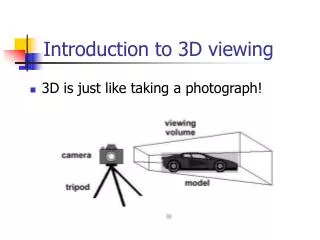
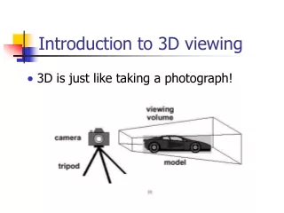
3D Viewing. Camera Analogy. 3D is just like taking a photograph (lots of photographs!) It uses transformations. viewing volume. camera. model. tripod. Camera Analogy and Transformations. Projection transformations adjust the lens of the camera Viewing transformations

E N D
Camera Analogy • 3D is just like taking a photograph (lots of photographs!) • It uses transformations viewing volume camera model tripod
Camera Analogy and Transformations • Projection transformations • adjust the lens of the camera • Viewing transformations • tripod–define position and orientation of the viewing volume in the world • Modeling transformations • moving the model • Viewport transformations • enlarge or reduce the physical photograph
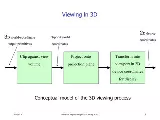
Coordinate Systems and Transformations • Steps in forming an image • specify geometry (world coordinates) • specify camera (camera coordinates) • project (window coordinates) • map to viewport (screen coordinates) • Each step uses transformations • Every transformation is equivalent to a change in coordinate systems (frames)
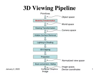
v e r t e x Modelview Matrix Projection Matrix Perspective Division Viewport Transform Modelview Projection Modelview l l l Transformation Pipeline • other calculations here • material è color • shade model (flat) • polygon rendering mode • polygon culling • clipping normalized device eye object clip window
Projection Transformation • Shape of viewing frustum • Perspective projection gluPerspective( fovy, aspect, zNear, zFar ) glFrustum(left,right,bottom,top,zNear,zFar) • Orthographic parallel projection glOrtho(left,right,bottom,top,zNear,zFar) gluOrtho2D( left, right, bottom, top ) • calls glOrtho with z values near zero
Applying Projection Transformations • Typical use (orthographic projection) glMatrixMode( GL_PROJECTION ); glLoadIdentity(); glOrtho(left, right, bottom, top, zNear, zFar);
tripod Viewing Transformations • Position the camera/eye in the scene • place the tripod down; aim camera • To “fly through” a scene • change viewing transformation andredraw scene gluLookAt( eyex, eyey, eyez, aimx, aimy, aimz, upx, upy, upz ) • up vector determines unique orientation
VRP - AT n = | VRP - AT | U U = VUP n, u = |U| n x u = v Viewing Specification & Eye Coordinates • Suppose that modeling transformation has been done and now all objects are in WC. • We need viewing specification or camera information. • VRP: view reference point or eye position. • AT: a reference point for objects. (ATis a reference point toward which the eye is aimed. AT is typically somewhere in the middle of the scene.) • VUP: view up vector. • VPN: view plane normal. (orientation of projection point) VRP-AT • {VRP, u, v, n} defines eye coordinates (EC), which is also called camera coordinates or view coordinates. • In EC, camera is at the origin and looks in the –n direction. y y VUP v VRP AT u n z z x x VRP
Eye Coordinates: Teapot Example • Let’s focus on the teapot centered at WC. v u n VRP
y y v v u u x x VRP n z z n Viewing Transformation • We have two coordinates: WC={O,x,y,z} and EC={VRP,u,v,n}. • Let’s superimpose EC onto WC: a translation followed by a rotation. • Such a transformation (which is a rigid motion) simply reinterprets the model from WC into EC, and is called viewing transformation. y v u VRP n x z
Viewing Transformation (cont’d) • viewing transformation in a single 4x4 matrix • Why from WC to EC? It’s for easy projection and clipping. You will see pretty soon! • Modeling and viewing transformations are often combined into a matrix Mmodelview. viewing transformation modeling transformation in WC in EC in LC modelview transformation in LC in EC
v y u x z n View Volume • Thanks to the viewing transformation, all vertices are newly defined in EC={VRP,u,v,n}, and we can forget about the WC={O,x,y,z}. • Then, let’s use {x,y,z} and {u,v,n} interchangeably because we are familiar with {x,y,z}. • Suppose a huge scene. In general, we cannot see all objects in the scene. We need to specify how much of the scene we can see. View volume does it. =
Perspective View Volume • We can imagine a window through which we can see the world. • The window is parallel to xy-plane. • Then, for perspective projection, the output image is made by the projectors (from COP) that pass through the window. • Such a perspective view volume makes an infinite pyramid. • We can bound near and far sides of the infinite pyramid. • The perspective view volume makes a truncated pyramid, frustum. • Only the objects inside the frustum are visible. y COP window z x window near plane far plane COP
Perspective View Volume (cont’d) • The frustum is defined by {l, r, b, t, n, f} which stands for {left, right, bottom, top, near, far}. We set n and fto be positive such that they are the perpendicular distances from COP to the two planes. • Note that the pyramid is not upright, which is unrealizable in the camera model but is useful for simulating human stereo vision, etc. z = -f -z y far plane near plane (r, t, -n) COP x (l, b, -n) z
Viewing Examples: Model and EC • Given the model in the figure, suppose that VRP=(0,0,40), AT=(0,0,0), and VUP=(0,10,0). • Let’s see some view volume examples with this model. y 10 VUP v=y=10 -n=-z AT 10 x v=y v 20 -20 30 -10 u=x=10 COP u u=x z=40 z n n=z
Perspective Projection Example I (60, 60, -40) • example 1 • We got the following image, where the viewport corresponds to the view volume’s window. 60 l= 0, r = 6 b = 0, t = 6 n = 4, f= 40 far plane 40 20 y=10 viewport x=10 20 40 60 near plane -20 (r, t, -n) = (6, 6, -4) COP (l, b, -n) = (0, 0, -4)
Perspective Projection Example II (60, 60, -40) • example 2 • What if the window size is reduced by 1/4? • We got the following image. 60 l= 0, r = 3 b = 0, t = 3 n = 4, f= 40 40 (30, 30, -40) 20 viewport 20 40 60 -20 (6, 6, -4) COP (3, 3, -4)
(22.5, 22.5, -15) Perspective Projection Example III (60, 60, -40) 60 • example 3 • What if the far plane moves towards COP? • We got the following image. l= 0, r = 6 b = 0, t = 6 n = 4, f= 15 40 20 viewport 20 40 60 -20 (6, 6, -4) COP
y x z Parallel Projection: Oblique vs. Orthographic • Recall that view plane and window are parallel to xy-plane. • Let’s consider the cross-section of EC (seen along –y direction). • Orthographic projection is a special parallel projection where the view plane is orthogonal to DOP. • perspective • parallel • - orthographic • - oblique x z Assuming the DOP is parallel to xz-plane. x x x DOP DOP DOP z orthographic oblique z z
DOP window Parallel View Volume • In parallel projection, the view volume is an infinite parallelepiped (not necessarily a box), which is parallel to DOP. • We can also bound near and far sides of the infinite parallelepiped to make the parallel view volume. (Imagine that the window slides along DOP to make both planes.) • Only the objects inside the view volume are visible. window near plane far plane
Parallel View Volume (cont’d) • Oblique projection is much less common, and so let’s consider only orthographic projection where DOP is orthogonal to the view plane. • Note that DOP is along the z-axis. • Then, the view volume has to be aligned with xyz-axes. • Two end points in a diagonal are enough to define the view volume. • As in the perspective projection, we set nand fto be positive. • Note that the view volume is defined by {l, r, b, t, n, f} for both perspective projection and orthographic projection. Of course, the set {l, r, b, t, n, f} has different semantics in the two cases. (r, t, -f) DOP y parallel view volume (l, b, -n) x z
y=10 -z y -20 -10 x=10 x z Orthographic Projection Examples • Let’s use the same example. • example 2 l= 0, r = 20 b = 0, t = 20 n = 15, f= 40 • example 3 l= 5, r = 20 b = 5, t = 20 n = 15, f= 40 • example 4 • example 1 l= 5, r = 20 b = 5, t = 20 n = 25, f= 40 l= 0, r = 20 b = 0, t = 20 n = 4, f= 40
Culling & Clipping • Where are we now? • Objects are defined in EC through modeling and viewing transformations. • Projection type (parallel or perspective) is specified. • View volume is given as {l, r, b, t, n, f} in EC. • The view volume specifies how much of the scene we can see. So, polygons completely inside the view volume are processed for display. • How about the scene outside the view volume? • Polygons completely outside the view volume are culled. • Polygons intersecting the boundary of the view volume are clipped against the boundary, and then processed for display.
Clipping: Teapot Example • Suppose that, in orthographic projection, we have a view volume intersecting the teapot. clipped polygon mesh to be rendered
y -1 -z 1 -1 1 x -x -1 z 1 -y Projection Transformation • OK, we just specified the view volume {l, r, b, t, n, f} in EC. The next step is projection transformation. • Let’s first tackle the orthographic projection. • Operations can be easily implemented in canonical view volume(CVV), which is defined as a 2x2x2 cube with its center at the origin, i.e. x=y=z=[-1,1]. • Projection transformation or specifically orthographic transformation transforms the box view volume into CVV.
y -1 -z 1 -1 1 x -x -1 z Tpar = 1 -y Projection Transformation (cont’d) • Obviously we need scaling. However, scaling is about origin. • As the 1st step, let’s translate the view volume’s center to the origin. • We know that the view volume’s center is ((l+r)/2,(b+t)/2,-(n+f )/2)). • So, the translation is Tpar = T(-(l+r)/2,-(b+t)/2,(n+f )/2)) y x=[-1,1] y=[-1,1] z=[-1,1] x=[l,r] y=[b,t] z=[-n,-f] x z y x Tpar makes z
Spar = Projection Transformation (cont’d) • Note that the CVV has the size of 2x2x2. So, let’s scale! • Width along x “r - l” should be scaled into 2. • So, scaling factor along x direction Sx = 2/(r-l) • Similarly, Sy = 2/(t-b) and Sz = 2/(f-n) • Mortho=Spar • Tpar is the orthographic (projection) transformation from the box view volume into CVV, or from EC to clip coordinates (CC). • After orthographic transformation, clipping is done. Then, the clipped model is within CVV whose dimensions are all 1 along x/y/z axes. It’s called that the model is in normalized devicecoordinates(NDC). • Some people say we have a 3D film (generated by projection). y x z r - l
Projection Transformation (cont’d) • Orthographic transformation with teapot example. v u n translation scaling CVV in NDC
Projection Transformation (cont’d) • Given {l, r, b, t, n, f}, the orthographic transformation Mortho is computed as Spar• Tpar. • Mortho can be simply rewritten as follows. x = (2/(r-l))x - (r+l)/(r-l) y = (2/(t-b))y - (t+b)/(t-b) z = (2/(f-n))z + (f+n)/(f-n)
Projection Transformation (cont’d) + • Some systems such as OpenGL use -z direction (0 0 -1) as DOP. (Compare this with positive-z projection direction in EC.) For this purpose, 3D reflection is required. reflection wrt xy-plane
Window Coordinates and Viewport • A window at your screen (not the window associated with the view volume) is associated with window coordinates (WdC). • A viewport is defined at WdC. • The viewport is not necessarily the entire window, and is defined by its lower left corner (xmin & ymin), width, and height. • Viewport transformation transforms the x- and y-coordinates of CVV to coincide with the viewport. viewport window height (xmin,ymin) width
viewport y oy y -1 height/2 z=-1 y -z ymin 1 x -1 1 x -x ox z xmin -1 x z -width/2 1 -y width/2 z -height/2 z=1 Viewport Transformation • The viewport transformation is a scaling followed by a translation. • For scaling, Sx=width/2 andSy=height/2. • Translation moves the center at the origin to the viewport center (ox,oy)=(xmin+width/2, ymin+height/2). • So, Mviewport= T(ox,oy,0) • S(Sx, Sy,1). Simply, x=x*(width/2)+ox and y=y*(height/2)+oy. Don’t do matrix multiplication. translation scaling
Viewport Transformation (cont’d) • Viewport transformation with teapot example • Final images CVV
Orthographic Projection Summary • The modeling transformation moves from LC to WC. • Viewing specifies the location/orientation of the viewer or camera, and viewing transformation moves from WC to EC. • The two transformations are combined into Mmodelview. • The view volume is defined by {l, r, b, t, n, f}. • The orthographic transformationMortho changes the view volume into CVV. It’s said the model is then in clip coordinates(CC). • Clipping is done. • The viewport transformationMviewport transforms vertices in CVV into 3D points in WdC. orthographic transformation modeling & viewing transformation in EC in LC viewport transformation in CC in WdC clipping in NDC
y -1 -z 1 -1 1 x -x -1 z 1 -y Projection Transformation for Perspective Projection • Now, let’s tackle the perspective projection • Note that the modelview transformation does not depend on the projection type. What distinguishes the perspective projection from the parallel projection is the projection transformation. • Perspective projection transformation: from the frustum to CVV. • It is often simply called a perspective transformation. -z z=-f y far plane (r, t, -n) near plane COP x (l, b, -n) z
-z -z z: unaffected x= x + pz should be x x 3D Shearing • Let’s see the frustum along -y direction • So, shearing along x is needed. OK, but is that it? No … -z z=-f y far plane (r, t, -n) near plane COP x (l, b, -n) z
y z: unaffected y = y + qz -z should be 3D Shearing (cont’d) y • Similarly, let us see along -x. • Hxy(p,q) makes the vector CC, which connects COP and the near plane’s center ((l+r)/2, (b+t)/2, -n), be (0, 0, -n). -z -z z=-f y far plane near plane (r, t, -n) COP x (l, b, -n) z x x+pz 1 0 p 0 Hxy(p,q) in summary z: unaffected x = x + pz y = y + qz y y+qz 0 1 q 0 = z z 0 0 1 0 1 1 0 0 0 1
3D Shearing (cont’d) • Let’s compute p and q. • If the frustum happens to be upright, CCx=CCy=0, and so p=q=0, which means that Hxy(p,q)= I and shearing has no effect. CC = near-plane-center - COP should be
Shearing followed by Scaling • 3D shearing has made the skewed frustum upright. • Now, let’s make the frustum’s side faces be of 45° slope. • Such a task can be performed by scaling. y y y To be done! 45° Done! -z -z -z original frustum upright frustum 45°-slope frustum
Scaling • Note that shearing does not change the size of the near plane. • Both (r-l)/2 and (t-b)/2 should be the same as n for making a 45°-slope frustum. We then need scaling! • Sx= n/[(r-l)/2] = 2n/(r-l) • Sy= n/[(t-b)/2] = 2n/(t-b) • Sz = 1. (r-l)/2 -z y (t-b)/2 near plane n x COP z
Shearing & Scaling: Teapot Example scaling shearing
Distortion • From the 45° frustum into CVV: Let’s represent (x2 y2 z2)in terms of(x1 y1 z1). y p -z1 y z=-f 1 n (x1,y1,z1) (x2,y2,z2) z z 1 -1 z1 -n z=-n -1 The point p (whose y value is -z1) should go to y=1. -z1:1 = y1: y2 y2= -y1/z1 Similarly, x2= -x1/z1
Distortion (cont’d) • We found that x2=-x1/z1 and y2=-y1/z1 . • How about z2? • We are to use matrix multiplication to represent projection. • z2= (ax1+by1+cz1+d)/(ex1+fy1+gz1+h) • (ex1+fy1+gz1+h)<- this part should be the same for x, y, and z • Z value should be independent of x, y value • Therefore z2= (cz1+d)/z1 • z2=A+B/z1. • OK, we found that z2=A+B/z1. • Let’s compute A and B. should be for the formula to be planar
Distortion (cont’d) • Let’s compute A and B for z2=A+B/z1. • Note that z1=[-f, -n] and z2=[-1,1]. • So, if z1= -f, then z2= -1. Similarly, if z1= -n, then z2=1. • Solving the two equations, we get A=(n+f)/(n-f) and B=2nf/(n-f). • (x2 y2 z2 1) = (-x1/z1 -y1/z1A+B/z11) = (x1 y1 -Az1-B -z1) • Multiplying every component by -z1, we can represent the distortion transformation “by a matrix multiplication.” • It’s possible thanks to homogeneous coordinate system. called Mdistort not (0 0 0 1) !!
y y z z x x Why called Distortion? • Mdistort distorts the model, and is not affine in the sense that parallelism is not preserved. • Distortion transformation moves COP to the position of z-axis. • The model is distorted, but leads to a correct image as we are now in (orthographic) CVV. into CVV model distortion
Perspective Division • In homogeneous coordinates, each vertex should be divided by its w-component to get a corresponding Cartesian coordinates. • It’s called perspective division. • An example n=1 f=2 A=(n+f)/(n-f) B=2nf/(n-f). y Q=(0 1 -1/3) Q=(0 3/2 –3/2) P=(0 1 1) 3/2 1 1/2 P=(0 1 -1) -z -2 R=(0 1/2 –3/2) R=(0 1/3 -1/3)
Perspective Division (cont’d) • The distortion transformation converts (x y z 1)into (x y -Az-B -z), and the perspective division is done by w=-z, which actually represents the distance from the eye. • As the distance from the eye increases, 1/w approaches 0, and so x/w and y/w also approach 0. This is how foreshortening is achieved. a b model distortion b a
Perspective Division (cont’d) • Observe that Q and R are at the center of the frustum along z-axis but Q and R are not at the center of CVV. • As the transformed z-coordinates move farther away from the near plane, the locations become increasingly less precise. Such a non-linearity caused by perspective division leads to some problem for hidden-surface removal. Let’s revisit this later. y Q=(0 1 -1/3) Q=(0 3/2 –3/2) P=(0 1 1) 3/2 1 1/2 P=(0 1 -1) -z -2 R=(0 1/2 –3/2) R=(0 1/3 -1/3)