Download
1 / 19
190 likes | 375 Views
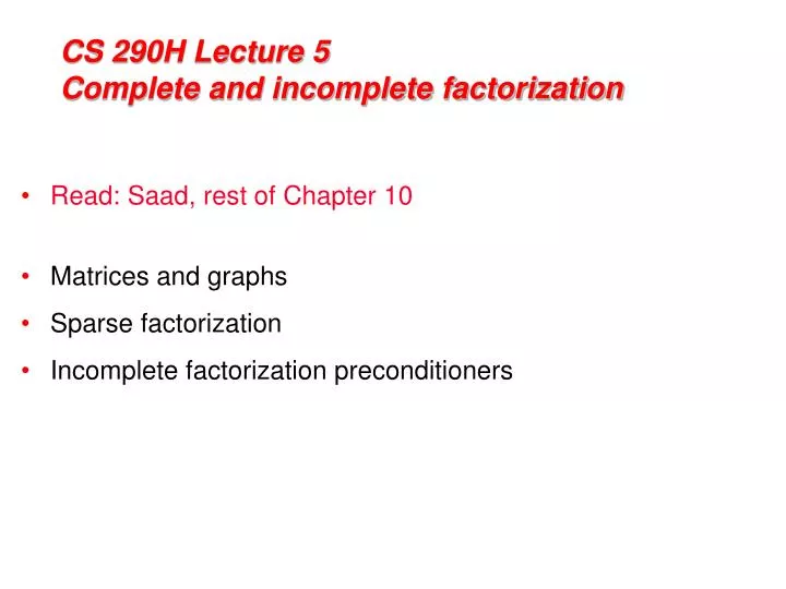
CS 290H Lecture 5 Complete and incomplete factorization. Read: Saad, rest of Chapter 10 Matrices and graphs Sparse factorization Incomplete factorization preconditioners. n 1/2. n 1/3. Complexity of linear solvers. Time to solve model problem (Poisson’s equation) on regular mesh. n 1/2.

E N D
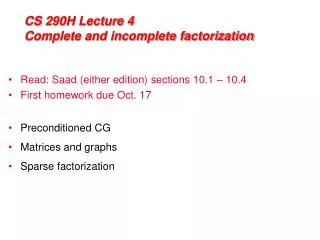
CS 290H Lecture 5Complete and incomplete factorization • Read: Saad, rest of Chapter 10 • Matrices and graphs • Sparse factorization • Incomplete factorization preconditioners
n1/2 n1/3 Complexity of linear solvers Time to solve model problem (Poisson’s equation) on regular mesh
n1/2 n1/3 Complexity of direct methods Time and space to solve any problem on any well-shaped finite element mesh
for j = 1 : n for k = 1 : j-1 % cmod(j,k) for i = j : n A(i,j) = A(i,j) – A(i,k)*A(j,k); end; end; % cdiv(j) A(j,j) = sqrt(A(j,j)); for i = j+1 : n A(i,j) = A(i,j) / A(j,j); end; end; j R RT A RT Column Cholesky Factorization: A=RTR • Column j of A becomes column j of RT
for j = 1 : n for k = 1 : j-1 % cmod(j,k) A(j:n, j) = A(j:n, j) – A(j:n, k)*A(j, k); end; % cdiv(j) A(j,j) = sqrt(A(j,j)); A(j+1:n, j) = A(j+1:n, j) / A(j,j); end; j R RT A RT Column Cholesky Factorization: A=RTR • Column j of A becomes column j of RT
Data structures • Full: • 2-dimensional array of real or complex numbers • (nrows*ncols) memory • Sparse: • compressed column storage • about (2*nzs + ncols) memory
for j = 1 : n for k < j with A(j,k) nonzero % sparse cmod(j,k) A(j:n, j) = A(j:n, j) – A(j:n, k)*A(j, k); end; % sparse cdiv(j) A(j,j) = sqrt(A(j,j)); A(j+1:n, j) = A(j+1:n, j) / A(j,j); end; j R RT A RT Sparse Column Cholesky Factorization: A=RTR • Column j of A becomes column j of RT
3 7 1 3 7 1 6 8 6 8 4 10 4 10 9 2 9 2 5 5 Graphs and Sparse Matrices: Cholesky factorization Fill:new nonzeros in factor Symmetric Gaussian elimination: for j = 1 to n add edges between j’s higher-numbered neighbors G+(A)[chordal] G(A)
Path lemma Let G = G(A) be the graph of a symmetric, positive definite matrix, with vertices 1, 2, …, n, and let G+ = G+(A)be the filled graph. Then (v, w) is an edge of G+if and only if G contains a path from v to w of the form (v, x1, x2, …, xk, w) with xi < min(v, w) for each i. (This includes the possibility k = 0, in which case (v, w) is an edge of G and therefore of G+.)
Sparse Cholesky factorization: A=RTR • Preorder • Independent of numerics • Symbolic Factorization • Elimination tree • Nonzero counts • Supernodes • Nonzero structure of R • Numeric Factorization • Static data structure • Supernodes use BLAS3 to reduce memory traffic • Triangular Solves
x A RT R Incomplete Cholesky factorization (IC, ILU) • Compute factors of A by Gaussian elimination, but ignore fill • Preconditioner B = RTR A, not formed explicitly • Compute B-1z by triangular solves (in time nnz(A)) • Total storage is O(nnz(A)), static data structure • Either symmetric (IC) or nonsymmetric (ILU)
1 4 1 4 3 2 3 2 Incomplete Cholesky and ILU: Variants • Allow one or more “levels of fill” • unpredictable storage requirements • Allow fill whose magnitude exceeds a “drop tolerance” • may get better approximate factors than levels of fill • unpredictable storage requirements • choice of tolerance is ad hoc • Partial pivoting (for nonsymmetric A) • “Modified ILU” (MIC): Add dropped fill to diagonal of U or R • A and RTR have same row sums • good in some PDE contexts
Incomplete Cholesky and ILU: Issues • Choice of parameters • good: smooth transition from iterative to direct methods • bad: very ad hoc, problem-dependent • tradeoff: time per iteration (more fill => more time)vs # of iterations (more fill => fewer iters) • Effectiveness • condition number usually improves (only) by constant factor (except MIC for some problems from PDEs) • still, often good when tuned for a particular class of problems • Parallelism • Triangular solves are not very parallel • Reordering for parallel triangular solve by graph coloring
Matrix permutations: Symmetric direct methods • Goal is to reduce fill, making Cholesky factorization cheaper. • Minimum degree: • Eliminate row/col with fewest nzs, add fill, repeat • Theory: can be suboptimal even on 2D model problem • Practice: often wins for medium-sized problems • Nested dissection: • Find a separator, number it last, proceed recursively • Theory: approx optimal separators => approx optimal fill and flop count • Practice: often wins for very large problems • Banded orderings (Reverse Cuthill-McKee, Sloan, . . .): • Try to keep all nonzeros close to the diagonal • Theory, practice: often wins for “long, thin” problems • Best orderings for direct methods are ND/MD hybrids.
Fill-reducing permutations in Matlab • Nonsymmetric approximate minimum degree: • p = colamd(A); • column permutation: lu(A(:,p)) often sparser than lu(A) • also for QR factorization • Symmetric approximate minimum degree: • p = symamd(A); • symmetric permutation: chol(A(p,p)) often sparser than chol(A) • Reverse Cuthill-McKee • p = symrcm(A); • A(p,p) often has smaller bandwidth than A • similar to Sparspak RCM D
Matrix permutations for iterative methods • Symmetric matrix permutations don’t change the convergence of unpreconditioned CG • Symmetric matrix permutations affect the quality of an incomplete factorization – poorly understood, controversial • Often banded (RCM) is best for IC(0) / ILU(0) • Often min degree & nested dissection are bad for no-fill incomplete factorization but good if some fill is allowed • Some experiments with orderings that use matrix values • e.g. “minimum discarded fill” order • sometimes effective but expensive to compute
Nonsymmetric matrix permutations for iterative methods • Dynamic permutation: ILU with row or column pivoting • E.g. ILUTP (Saad), Matlab “luinc” • More robust but more expensive than ILUT • Static permutation: Try to increase diagonal dominance • E.g. bipartite weighted matching (Duff & Koster) • Often effective; no theory for quality of preconditioner • Field is not well understood, to say the least
1 2 3 4 5 1 4 1 5 2 2 3 3 3 1 4 2 4 5 PA 5 Row permutation for heavy diagonal [Duff, Koster] 1 2 3 4 5 • Represent A as a weighted, undirected bipartite graph (one node for each row and one node for each column) • Find matching (set of independent edges) with maximum product of weights • Permute rows to place matching on diagonal • Matching algorithm also gives a row and column scaling to make all diag elts =1 and all off-diag elts <=1 1 2 3 4 5 A
A B-1 Sparse approximate inverses • Compute B-1 A explicitly • Minimize || A B-1 – I ||F (in parallel, by columns) • Variants: factored form of B-1, more fill, . . • Good: very parallel, seldom breaks down • Bad: effectiveness varies widely