The Influence of loss saturation effects on the assessment of polar ozone changes

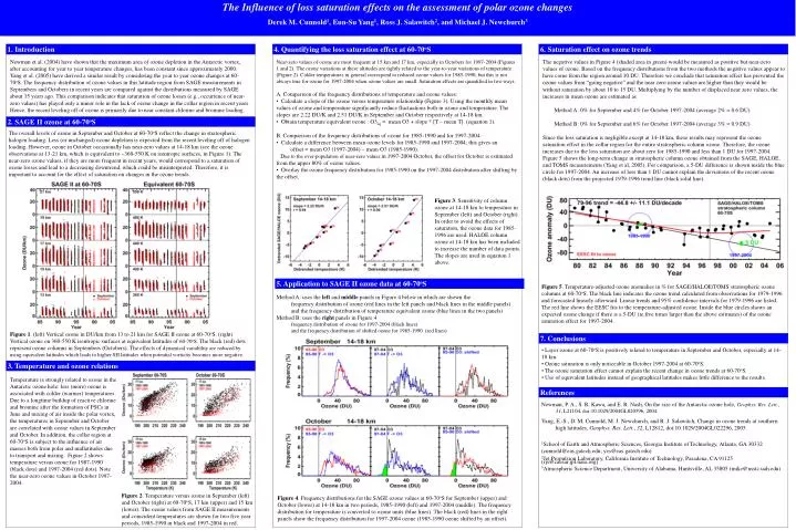
1. The Influence of loss saturation effects on the assessment of polar ozone changes Derek M. Cunnold1, Eun-Su Yang1, Ross J. Salawitch2, and Michael J. Newchurch3 1. Introduction 4. Quantifying the loss saturation effect at 60-70oS 6. Saturation effect on ozone trends Newman et al. (2004) have shown that the maximum area of ozone depletion in the Antarctic vortex, after accounting for year to year temperature changes, has been constant since approximately 2000. Yang et al. (2005) have derived a similar result by considering the year to year ozone changes at 60-70oS. The frequency distribution of ozone values in this latitude region from SAGE measurements in Septembers and Octobers in recent years are compared against the distributions measured by SAGE about 15 years ago. This comparison indicates that saturation of ozone losses (e.g., occurrence of near-zero values) has played only a minor role in the lack of ozone change in the collar region in recent years. Hence, the recent leveling off of ozone is primarily due to near constant chlorine and bromine loading. The negative values in Figure 4 (shaded area in green) would be measured as positive but near-zero values of ozone. Based on the frequency distributions from the two methods the negative values appear to have come from the region around 10 DU. Therefore we conclude that saturation effect has prevented the ozone values from “going negative” and the near zero ozone values are higher than they would be without saturation by about 10 to 15 DU. Multiplying by the number of displaced near zero values, the increases in mean ozone are estimated as Method A: 0% for September and 4% for October 1997-2004 (average 2% = 0.6 DU) Method B: 0% for September and 6% for October 1997-2004 (average 3% = 0.9 DU) Since the loss saturation is negligible except at 14-18 km, these results may represent the ozone saturation effect in the collar region for the entire stratospheric column ozone. Therefore, the ozone increases due to the loss saturation are about zero for 1985-1990 and less than 1 DU for 1997-2004. Figure 5 shows the long-term change in stratospheric column ozone obtained from the SAGE, HALOE, and TOMS measurements (Yang et al, 2005). For comparison, a 5-DU difference is shown inside the blue circle for 1997-2004. An increase of less than 1 DU cannot explain the deviations of the recent ozone (black dots) from the projected 1979-1996 trend line (black solid line). • Near-zero values of ozone are most frequent at 15 km and 17 km, especially in Octobers for 1997-2004 (Figures 1 and 2). The ozone variations at these altitudes are tightly related to the year-to-year variations of temperature (Figure 2). Colder temperatures in general correspond to reduced ozone values for 1985-1990, but this is not always true for ozone for 1997-2004 when ozone values are small. Saturation effects are quantified in two ways. • A. Comparison of the frequency distributions of temperature and ozone values: • Calculate a slope of the ozone versus temperature relationship (Figure 3). Using the monthly mean values of ozone and temperature significantly reduce fluctuations both in ozone and temperature. The slopes are 2.22 DU/K and 2.51 DU/K in September and October respectively at 14-18 km. • Obtain temperature equivalent ozone : O3eq = mean O3 + slope * [T – mean T] (equation 1). • B. Comparison of the frequency distributions of ozone for 1985-1990 and for 1997-2004: • Calculate a difference between mean ozone levels for 1985-1990 and 1997-2004; this gives an • offset = mean O3 (1997-2004) – mean O3 (1985-1990). • Due to the over-population of near-zero values in 1997-2004 October, the offset for October is estimated from the upper 80% of ozone values. • Overlay the ozone frequency distribution for 1985-1990 on the 1997-2004 distribution after shifting by the offset. 2. SAGE II ozone at 60-70oS The overall levels of ozone in September and October at 60-70oS reflect the change in stratospheric halogen loading. Less (or unchanged) ozone depletion is expected from the recent leveling off of halogen loading. However, ozone in October occasionally has near-zero values at 14-18 km (see the ozone observations at 13-21 km, which is equivalent to ~360-550 K on isentropic surfaces, in Figure 1). The near-zero ozone values, if they are more frequent in recent years, would correspond to a saturation of ozone losses and lead to a decreasing downtrend, which could be misinterpreted. Therefore, it is important to account for the effect of saturation on changes in the ozone trends. Figure 3. Sensitivity of column ozone at 14-18 km to temperature in September (left) and October (right). In order to avoid the effects of saturation, the ozone data for 1985-1996 are used. HALOE column ozone at 14-18 km has been included to increase the number of data points. The slopes are used in equation 1 above. 5. Application to SAGE II ozone data at 60-70oS Figure 5. Temperature-adjusted ozone anomalies in % for SAGE/HALOE/TOMS stratospheric ozone columns at 60-70oS. The black line indicates the ozone trend calculated from observations for 1979-1996 and forecasted linearly afterward. Linear trends and 95% confidence intervals for 1979-1996 are listed. The red line shows the EESC fits to the temperature-adjusted ozone. Inside the blue circles shows an expected ozone change if there is a 5-DU (ie.five times larger than the above estimates) of the ozone saturation effect for 1997-2004. Method A: uses the left and middle panels in Figure 4 below in which are shown the frequency distribution of ozone (red lines in the left panels and black lines in the middle panels) and the frequency distribution of temperature equivalent ozone (blue lines in the two panels) Method B: uses the right panels in Figure 4 frequency distribution of ozone for 1997-2004 (black lines) and the frequency distribution of shifted ozone for 1985-1990 (red lines) Figure 1. (left) Vertical ozone in DU/km from 13 to 21 km for SAGE II ozone at 60-70oS. (right) Vertical ozone on 360-550 K isentropic surfaces at equivalent latitudes of 60-70oS. The black (red) dots represent ozone columns in Septembers (Octobers). The effects of dynamical variability are reduced by using equivalent latitudes which leads to higher SH latitudes when potential vorticity becomes more negative. 7. Conclusions • Layer ozone at 60-70oS is positively related to temperature in September and October, especially at 14-18 km. • Ozone saturation is only noticeable in October 1997-2004 at 60-70oS. • The ozone saturation effect cannot explain the recent change in ozone trends at 60-70oS. • Use of equivalent latitudes instead of geographical latitudes makes little difference to the results. 3. Temperature and ozone relations Temperature is strongly related to ozone in the Antarctic ozone hole: less (more) ozone is associated with colder (warmer) temperatures. Due to a longtime buildup of reactive chlorine and bromine after the formation of PSCs in June and mixing of air inside the polar vortex, the temperatures in September and October are correlated with ozone values in September and October. In addition, the collar region at 60-70oS is subject to the influence of air masses both from polar and midlatitudes due to transport and mixing. Figure 2 shows temperature versus ozone for 1987-1990 (black dots) and 1997-2004 (red dots). Note the near-zero ozone values in October 1997-2004. References Newman, P. A., S. R. Kawa, and E. R. Nash, On the size of the Antarctic ozone hole, Geophys. Res. Lett., 31, L21104, doi:10.1029/2004GL020596, 2004. Yang, E.-S., D. M. Cunnold, M. J. Newchurch, and R. J. Salawitch, Change in ozone trends at southern high latitudes, Geophys. Res. Lett., 32, L12812, doi:10.1029/2004GL022296, 2005. 1School of Earth and Atmospheric Sciences, Georgia Institute of Technology, Atlanta, GA 30332 (cunnold@eas.gatech.edu; yes@eas.gatech.edu) 2Jet Propulsion Laboratory, California Institute of Technology, Pasadena, CA 91125 (rjs@caesar.jpl.nasa.org) 3Atmospheric Science Department, University of Alabama, Huntsville, AL 35805 (mike@nsstc.uah.edu) Figure 2. Temperature versus ozone in September (left) and October (right) at 60-70oS, 17 km (upper) and 15 km (lower). The ozone values from SAGE II measurements and coincident temperatures are shown for two five year periods, 1985-1990 in black and 1997-2004 in red. Figure 4. Frequency distributions for the SAGE ozone values at 60-70oS for September (upper) and October (lower) at 14-18 km in two periods, 1985-1990 (left) and 1997-2004 (middle). The frequency distribution for temperature is converted to ozone units (blue lines). The black (red) lines in the right panels show the frequency distribution for 1997-2004 ozone (1985-1990 ozone shifted by an offset).