Download
1 / 40
400 likes | 499 Views
Searching for photons in the LAT. Francesco Longo Elisabetta Bissaldi University & INFN Trieste, Italy. Overview. Searching for photons in cosmic ray data Description of simple selection cuts (see Elisabetta, IA5) Analysis of 8 and 16 Towers configurations

E N D
Searching for photons in the LAT Francesco Longo Elisabetta Bissaldi University & INFN Trieste, Italy
Overview • Searching for photons in cosmic ray data • Description of simple selection cuts (see Elisabetta, IA5) • Analysis of 8 and 16 Towers configurations • Application of DC2 cuts • Preliminary analysis with R.Rando’s random forests program • Conclusions
g m W W SI SI SI SI e+ e- Ground Analysis Cosmic Ray Muons Cosmic Ray Photon Candidates Event Display: 8 Towers
Extended analysis (see IA5) Used only “VERTEX” topology Searched for further selections analysing important variables 2, 4, and 6 towers configurations Deepened the analysis by studying different vertex topologies Original idea (see IA3) Analysis of Monte Carlo samples to study Photons and Muons distributions Initial selection cuts Definition of 2 g topologies VtxAngle>0. “VERTEX” VtxAngle=0. “1TRACK” Development of an algorithm based on classification trees Study of relative importance of variables for selection Application of the algorithm to cosmic ray data collected with a single tower configuration (RUN 1338) Photon Candidate Selection Bill Atwood (march 2005) Elisabetta (august 2005) new: 8 and 16
Example of variable selection: “Tkr1SSDVeto” • Tkr1SSDVeto≡ Number of silicon planes between the top of the extrapolated track and the first plane that has a hit near the track. Only planes that have wafers which intersect the extrapolated track are considered. Can be used as a back-up for the ACD. • Selection: At least 1 plane before start of track Track projection Found track Tkr1SSDVeto>1
MC AllGamma 2, 4, 6, 8 Towers 1 x 10⁶ simul. events Isotropic 18 MeV – 18 GeV [v5r0608p7] 16 Towers 4 x 10⁶ simul. events 10 MeV – 20 GeV [v5r0703p4] MC Muons 2, 4, 6, 8 Towers 4 x 10⁶ simul. events Isotropic PDG formula and low energy extension [v5r0608p7] 16 Towers [v5r0703p4] MonteCarlo and DATA samples DATA Cosmic Rays • 2 Towers: RUN 135002134 (462678 triggered events) [v5r0608p6] • 4 Towers: RUN 135002778 (61996 trig. events) [v4r060302p23] • 6 Towers: RUN 135004075 (390035 trig. events) [v5r0608p6] • 8 Towers: RUN 135004453 (510562 trig. events) [v5r0608p6] • 16 Towers: RUN 135005345 (470286 trig. events) [v5r0703p4]
2, 4, 6, 8 and 16 Towers Results Final Selections (cumulative): • TkrNumTracks>0 • CalEnergySum>10. • VtxAngle>0. • Tkr1ToTFirst>1 • Tkr1SSDVeto>2 • Tkr1ToTTrAve>1.3
2 Towers Results 100 % 10 % 1 % 0.1 % 0.01 % MC AllGamma MC Muons DATA Final Selections (cumulative): • TkrNumTracks>0 • CalEnergySum>10. • VtxAngle>0. • Tkr1ToTFirst>1. • Tkr1SSDVeto>1 • Tkr1ToTTrAve>1.3 STEPS 1. 2. 3. 4. 5. 6.
16 Towers Results 100 % 10 % 1 % 0.1 % 0.01 % MC AllGamma DATA Final Selections (cumulative): • TkrNumTracks>0 • CalEnergySum>10. • VtxAngle>0. • Tkr1ToTFirst>1. • Tkr1SSDVeto>1 • Tkr1ToTTrAve>1.3 • VtxStatus = 162 MC Muons STEPS 1. 2. 3. 4. 5. 6. 7.
Photon Sample from Elisabetta’s analysis DATA 2Towers MC Photons 2Towers CalEnergySum CalEnergySum NEW cuts NEW cuts ~1% of initial triggers N° events N° events Energy in MeV Energy in MeV TkrNumTracks > 0 CalEnergySum > 10. VtxAngle > 0. Tkr1TotFirst > 1. Tkr1SSDVeto > 1 Tkr1ToTTrAve > 1.3 VtxStatus = 162 Extrapolate these numbers for full LAT we expect a factor of 100 more photon candidates in the next data set Should we apply Elisabetta’s cuts and create a photon sample for everyone?
1 162 0 162 34 128 86 % 6 % 3 % 59 % 13 % 7 % VtxStatus Distribution DATA 2 Towers NEW cuts no cuts 162 0 and 1 N° events N° events VtxStatus Value VtxStatus Value 0.6 % of initial triggers!
VtxStatus 162 g dir g dir hit W hit SI SI tracks tracks VtxStatus = 162 2 tracks vertex, vertex tracks share first hit and DOCA point lies inside track hits
AcdActiveDist3D No Cuts Simple Cuts
How to get CTB variables in? • Take original merit file • Use GlastClassify executable file “apply.exe” • Recalculates the CTB variables and fill the ntuples • No need for reading back the recon file • This will be needed if we asked also for “Onboard” filter type variables
“DC2” Cuts • TCut DC2Trigger="(GltWord&10)>0&&(GltWord!=35)"; • //TCut DC2Filter="FilterStatus_HI==0"; • TCut DC2PrefilterCal="CalEnergyRaw>5&&CalCsIRLn>4"; • TCut DC2AcdVeto="(AcdCornerDoca>-5&&AcdCornerDoca<50&&CTBTkrLATEdge<100)||((AcdActiveDist3D>0 || AcdRibbonActDist>0)&&Tkr1SSDVeto<2)"; // Filter out high energy electrons • TCut DC2ElectronVeto="((min(abs(Tkr1XDir),abs(Tkr1YDir)) < .01 && Tkr1DieEdge < 10 && AcdActiveDist3D > 0) || (Tkr1SSDVeto < 7 && AcdActiveDist3D > -3) || ( AcdActiveDist3D >(-30 + 30*(Tkr1FirstLayer-2)))) && (CTBGAM+0.17*CTBBestLogEnergy)<1.75"; // Filter out some events at low-med energy where the Track 2 starts higher up than Track 1. • TCut DC2AnotherVeto="(Tkr1FirstLayer - Tkr2FirstLayer) < 0 && Tkr2FirstLayer > 2 && Tkr2TkrHDoca>10 && (CTBGAM+0.16*CTBBestLogEnergy)<1.32 "; Following Bill and Julie presentations at C&A group
“DC2” Cuts // Heavy Ion Filter • TCut HeavyIonVeto = "CTBBestEnergy>1000 && (((CalTransRms-1.5)*Tkr1ToTTrAve)<5)&&CTBGAM>0.5"; // Anti-correlated filter • TCut AntiCorrVeto = "CTBBestEnergy<500&&((CalCsIRLn+2.5*Tkr1CoreHC/Tkr1Hits)<8 || (Tkr1CoreHC/Tkr1Hits)<0.03)"; //Cosmic proton filter • TCut ProtonVeto = "Tkr1FirstLayer<6&&AcdActiveDist3D>-80 && ((AcdActiveDist3D/100)>1)"; //Global Ribbon Extension and AcdCornerDoca Extension • TCut GlobalRibbonVeto = "(AcdRibbonActDist > -10) || (AcdCornerDoca >-5 && AcdCornerDoca<50 &&CTBTkrLATEdge<200)"; • TCut DC2Vetos = DC2AcdVeto||DC2ElectronVeto||DC2AnotherVeto||HeavyIonVeto||AntiCorrVeto|| ProtonVeto||GlobalRibbonVeto; • TCut Basic = "CTBCORE>0.1&&CTBBestEnergyProb>0.1&&CTBGAM>0."; • TCut ratecut = "CTBBestZDir<-0.3&&CTBBestEnergy>100.";
“DC2” Cuts • TCut DC2Base1 = "CTBCORE>0.1 &&CTBBestEnergyProb>0.3 &&CTBGAM>0.35"; • TCut DC2Base2 = "CTBCORE>0.1 &&CTBBestEnergyProb>0.1 &&CTBGAM>0.55"; • TCut DC2Base3 = "CTBCORE>0.35 &&CTBBestEnergyProb>0.35 &&CTBGAM>0.50"; // Final Analysis Classes • TCut GoodEvent1=(DC2Base1&&DC2Trigger&&DC2PrefilterCal)&&!DC2Vetos; • TCut GoodEvent3=(DC2Base3&&DC2Trigger&&DC2PrefilterCal)&&!DC2Vetos; // For DC2 we propose using the GoodEvent1 and GoodEvent3 analysis classes. • TCut EventClassA = GoodEvent3; • TCut EventClassB = GoodEvent1&&!GoodEvent3;
Results CalEnergyRaw CalEnergyRaw VtxStatus VtxStatus Simple Cuts “DC2” EventClass A and B
Results CalEnergyRaw VtxStatus Simple Cuts “DC2” EventClass A and B
Results CalEnergyRaw VtxStatus Simple Cuts “DC2” EventClass A and B
Analysis with rForest(random forest package developed by R.Rando)
How to do that? • Package available in /users/rando/rForest • Actually tag v2r1p2 • Two executables + some utilities • Create two sets of data (gamma and muon sample) • fcreate.exe takes the input merit files of the classes to be analysed and create the selection tree file • More details on rForest could be found at Riccardo’s tutorial at the INFN GLAST SW meeting http://glast.ba.infn.it/~glast/f2f/bari2_rando.pdf • fprocess.exe calculates the result for each event
Results CalEnergyRaw VtxStatus Simple Cuts rForest (not optimized)Cuts NB. Different surface muons file (due to a technical problem)
Results CalEnergyRaw VtxStatus Simple Cuts rForest (not optimized)Cuts
Results CalEnergyRaw VtxStatus Simple Cuts rForest (not optimized)Cuts
Plot of overall distributionsin “photon samples” Preliminary analysis
Simple Cuts (1) Results (6930 evts) GltGemSummary CalEnergyRaw VtxStatus CalMipNum
“DC2” (2) results (4392 evts) GltGemSummary CalEnergyRaw VtxStatus CalMipNum
rForest (3) Results (19565 evts) GltGemSummary CalEnergyRaw VtxStatus CalMipNum
Simple Cuts (1) results CalMIPRatio AcdNoTop AcdActiveDist3D AcdTileCount
“DC2” (2) results CalMIPRatio AcdNoTop AcdActiveDist3D AcdTileCount
rForest (3) Results CalMIPRatio AcdNoTop AcdActiveDist3D AcdTileCount
To Do List • Refine rForest analysis • Try GlastClassify analysis • Closer look to selected photon candidates • Deeper use of ACD and CAL variables • Analysis of selected distributions • Redo for FSW • Reanalysis of “muon” recon candidates
Conclusions • Simple selection cuts seem to be satisfactory • Need to develop ad hoc selection trees • Simple analysis performed • Need to continue with other runs
TkrNumTracks CalEnergyRaw Tkr1ToTFirst Tkr1ToTTrAve VtxAngle VtxStatus Tkr1SSDVeto Variables’ Importance