Download
1 / 30
300 likes | 433 Views
Last Time. Re-using paths Irradiance Caching Photon Mapping. Today. Radiosity A very important method in practice, because it is so much more efficient than Monte Carlo for diffuse environments

E N D
Last Time • Re-using paths • Irradiance Caching • Photon Mapping © 2005 University of Wisconsin
Today • Radiosity • A very important method in practice, because it is so much more efficient than Monte Carlo for diffuse environments • Can also be used in conjunction with Monte Carlo, if you’re very careful about partitioning the LTE into different components © 2005 University of Wisconsin
Radiosity • Radiosity is the total power leaving a surface, per unit area on the surface • Usually denoted B • The outgoing version of irradiance • To get it, integrate radiance over the hemisphere of outgoing directions: © 2005 University of Wisconsin
Exitance • Light sources emit light, they are sources of radiance • Exitance is the equivalent of radiosity for emitters: • Distinguish exitance from radiosity to simplify equations • Different from Intensity, which is power per unit solid angle • Exitance is not ill-defined for point light sources © 2005 University of Wisconsin
Radiosity Algorithms • Radiosity algorithms solve the global illumination equation under a restrictive set of assumptions • All surfaces are perfectly diffuse • We only care about the radiosity at surfaces • Some form of rendering pass is required to transfer to the image plane • Surfaces can be broken into patches with constant radiosity • Some algorithms extend this to linear combinations of basis functions • These assumptions allow us to linearize the global illumination equation © 2005 University of Wisconsin
Diffuse Surface Radiosity • Diffuse surfaces, by definition, have outgoing radiance that does not depend on direction • Same can be said for diffuse emitters • And recall the definition of the diffuse BRDF in terms of directional hemispheric reflectance © 2005 University of Wisconsin
Radiosity Light Transport • Simplifying the global illumination equation gives: • We have removed almost all the angular dependence, but we still have an integral of directions computing irradiance © 2005 University of Wisconsin
Switch the Domain • We can convert the integral over the hemisphere of solid angles into one over all the surfaces in a scene: © 2005 University of Wisconsin
Discretize Radiosity • Assume world is broken into N disjoint patches, Pi, i=1..N, each with area Ai • Assume radiosity is constant over patches • Define: © 2005 University of Wisconsin
Discrete Formulation • Change the integral over surfaces to a sum over patches: © 2005 University of Wisconsin
The Form Factor • Note that we use it the other way: the form factor Fijis used in computing the energy arriving at I • Also called the configuration factor Fij is the proportion of the total power leaving patch Pi that is received by patch Pj © 2005 University of Wisconsin
Form Factor Properties • Depends only on geometry • Reciprocity: AiFij=AjFji • Additivity: Fi(jk)=Fij +Fik • Reverse additivity is not true • Sum to unity (all the power leaving patch i must get somewhere): © 2005 University of Wisconsin
The Discrete Radiosity Equation • This is a linear equation! • Dimension of M is given by the number of patches in the scene: NxN • It’s a big system • But the matrix M has some special properties © 2005 University of Wisconsin
Solving for Radiosity • First compute all the form factors • These are view-independent, so for many views this need only be done once • Many ways to compute form factors • Compute the matrix M • Solve the linear system • A range of methods exist • Render the result using Gourand shading, or some other method – but no additional lighting, it’s baked in • Each patch’s diffuse intensity is given by its radiosity © 2005 University of Wisconsin
Solving the Linear System • The matrix is very large – iterative methods are preferred • Start by expressing each radiance in terms of the others: © 2005 University of Wisconsin
Relaxation Methods • Jacobi relaxation: Start with a guess for Bi, then (at iteration m): • Gauss-Siedel relaxation: Use values already computed in this iteration: © 2005 University of Wisconsin
Gauss-Seidel Relaxation • Allows updating in place • Requires strictly diagonally dominant: • It can be shown that the matrix M is diagonally dominant • Follows from the properties of form factors © 2005 University of Wisconsin
Displaying the Results • Color is handled by discretizing wavelength and solving each channel separately • Smooth shading: • Patch radiosities are mapped to vertex colors by averaging the radiosities of the patches incident upon the vertex • Per-vertex colors then used to Gourand shade © 2005 University of Wisconsin
Value for Computation • Most of the time is spent computing form factors - must solve N visibility problems • However, same form factors for different illumination conditions, and no color dependence • Result is view independent - have radiosities for all patches. May be good or may be wasteful © 2005 University of Wisconsin
Form Factors • Computing form factors means solving an integral • We have had plenty of practice at this kind of thing • Also a point-patch form: the proportion of the power from a differential area about point x received by j © 2005 University of Wisconsin
Form Factor Computations • Unoccluded patches: • Direct integration • Conversion to contour integration • Form factor algebra – set operations on areas correspond to numerical operations on form factors – not really useful • Occluded patches: • Monte Carlo integration • Projection methods (essentially numerical quadrature) • Hemisphere • Hemicube © 2005 University of Wisconsin
Direct Integration – e.g. Rect-Rect • Note that we can do this only under the constant radiosity over patch assumption • There is a formula for 2 isolated polygons, but it assumes they can see each other fully! © 2005 University of Wisconsin
Contour Integral • Use Stokes’ theorem to convert the area integrals into contour integrals • For point to polygon form factors, the contour integral is not too hard • Care must be taken when r0 © 2005 University of Wisconsin
Projection Methods • For patches that are far apart compared to their areas, the inner integral in the form factor doesn’t vary much • That is, the form factor is similar from most points on a surface i • So, compute point to patch form factors and weigh by area © 2005 University of Wisconsin
Nusselt’s Analogy • Integrate over visible solid angle instead of visible patch area: Fx,P is the fraction of the area of the unit disc in the base plane obtained by projecting the surface patch P onto the unit sphere centered at x and then orthogonally down onto the base plane. © 2005 University of Wisconsin
Same Projection – Same Form Factor • Any patches with the same projection onto the hemisphere have the same form factor • Makes sense: put yourself at the point and look out – if you see equal amounts, they get equal power • It doesn’t matter what you project onto: two patches that project the same have the same form factor © 2005 University of Wisconsin
Monte-Carlo Form Factors • We can use Monte-Carlo methods to estimate the integral over visible solid angle • Simplest method – cosine weighted sampling: • Sample the disc about the point • Project up onto the hemisphere, then cast a ray out from the point in that direction • Form factor for each patch is the weighted sum of the number of rays that hit the patch • There are even better Monte-Carlo methods that we will see later © 2005 University of Wisconsin
The Hemicube • We have algorithms, and even hardware, for projecting onto planar surfaces • The hemicube consists of 5 such faces • A “pixel” on the cube has a certain projection, and hence a certain form factor • Something that projects onto the pixel has the same form factor © 2005 University of Wisconsin
Hemicube, cont. • Pretend each face of the hemicube is a screen, and project the world onto it • Code each polygon with a color, and count the pixels of each color to determine C(j) • Quality depends on hemicube resolution and z-buffer depth © 2005 University of Wisconsin
Next Time • Progressive Radiosity © 2005 University of Wisconsin