Download
1 / 25
250 likes | 353 Views
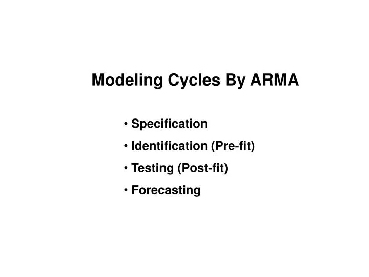
Modeling Cycles By ARMA. Specification Identification (Pre-fit) Testing (Post-fit) Forecasting. Definitions. Data =Trend + Season+Cycle + Irregular Cycle + Irregular = Data – Trend – Season (curves) (dummy variables) For this presentation, let: Y t = Cycle t + Irregular t.

E N D
Modeling Cycles By ARMA • Specification • Identification (Pre-fit) • Testing (Post-fit) • Forecasting
Definitions • Data =Trend + Season+Cycle + Irregular • Cycle + Irregular = Data – Trend – Season(curves) (dummy variables) • For this presentation, let: Yt = Cyclet + Irregulart
Stationary Process For Cycles Cycle + Irregular =(A) Stationary Process =(A) ARMA(p, q) =(A) : Approximation
Stationary Process • Series Yt is stationary if:mt = m, constant for all t st = s, constant for all t r(Yt, Yt+h) = rh does not depend on t • WN is a special example of a stationary process
Models For a Stationary Process • Autoregressive Process, AR(p) • Moving Average Process, MA(q) • Autoregressive Moving Average Process, ARMA(p, q)
Parameters of ARMA Models Specification Parameters fk Autoregressive Process Parameter qkMoving Average Process Parameter Characterization Parameters rk Autocorrelation Coefficient fkk Partial Autocorrelation Coefficient
AR Process • AR (1) : (Yt - m ) = f1 (Y(t-1) - m ) + e t -1 < f1 < 1 (stationarity condition) • AR (2) :(Yt - m) = f1 (Y(t-1) - m) + f2 (Y(t-2) - m ) + e t f2 + f1 < 1, f2 - f1 < 1 , -1 < f2 < 1 (stationarity condition) e t is a WN (s)
MA Process • MA (1) : Yt - m = et + q 1 e(t-1) - 1 < q1 < 1 (invertibility condition) • MA (2) : Yt - m = et + q 1 e (t-1) + q2 e (t-2) q2 + q1 >-1, q2 - q1 >- 1 , -1 < q2 < 1 (invertibility condition) e t is a WN (s)
ARMA (p, q) Models • ARMA(1, 1): (Yt - m ) = f1 (Y(t-1) - m ) + e t + q 1 e(t-1) • ARMA(2, 1): (Yt - m ) = f1 (Y(t-1) - m ) + f2 (Y(t-2) - m ) + e t + q 1 e(t-1) • ARMA(1, 2): (Yt - m ) = f1 (Y(t-1) - m ) + e t + q 1 e(t-1) + q 2 e(t-2)
Wold Theorem • Any “stationary process” can be defined as a linear combination of a WN series, et means: with: sum( ) < inf.
Lag Operator, L • Lag Operator, L • Then, the Wold Theorem can be written as:
Approximation • Approximation of B(L) by a Simple Rational Polynomial of L
Generating AR(1) • Let:
Generating MA(1) • Let:
Generating ARMA(1,1) • Your Exercise
AR, MA or ARMA?Pre-Fitting Model Identification • Using ACF and PACF
Partial Autocorrelation Function:PACF • Notation: • The partial autocorrelation of order k is denoted as f kk • Interpretation: f kk = Correlation (Yt, Y(t-k) Y(t-1) ,..., Y(t-k+1) ) Yt, {Y(t-1), Y(t-2), ... , Y(t-k+1)}, Y(t-k)
Patterns of ACF and PACF • AR processes • MA processes • ARMA processes
Model Diagnostics – Post Fit • Residual Check: • Correlogram of the Residual • QLB Statistic (m - # of parameters) • SE • Test of Significance of Coefficients • AIC, SIC
AIC and SIC (Maximized) (Minimized)
Truth is Simple • Parsimony • Use a minimum number of unknown parameters
Importance of Parsimony • In-Sample RMSE (SE) of Model Prediction vs. B. Out-of-Sample RMSE The two should not differ much.
Eview Commands • AR • ls series_name c ar(1) ar(2).. • MA • ls series_name c ma(1) ma(2).. • ARMA • ls series_name c ar(1) ar(2)….ma(1) ma(2)….
Forecasting Rules • Sample range: 1 to T. Forecast T+h for h=1,2,… • Write the model, with all unknown parameters replaced by their estimates. • Write the information set WT (only necessary part) • The unknown errors are given 0. • Use the chain rule.
Interval Forecast • h=1 • Use SE of Regression for setting the upper and the lower limits • h=2 • a) AR(1) • b) MA(1) • c) ARMA(1,1)