Download
1 / 52
520 likes | 616 Views
CALIBRATION OF A TRANSPORT MODEL USING DRIFTING BUOYS DEPLOYED DURING THE PRESTIGE ACCIDENT S. CASTANEDO, A.J. ABASCAL, R. MEDINA and I.J. LOSADA. OUTLINE. 1. Introduction Data Methodology 4. Conclusions. OUTLINE. 1. Introduction Data Methodology 4. Conclusions.

E N D
CALIBRATION OF A TRANSPORT MODEL USING DRIFTING BUOYS DEPLOYED DURING THE PRESTIGE ACCIDENT S. CASTANEDO, A.J. ABASCAL, R. MEDINA and I.J. LOSADA
OUTLINE • 1. Introduction • Data • Methodology • 4. Conclusions
OUTLINE • 1. Introduction • Data • Methodology • 4. Conclusions
1. INTRODUCTION • Along the Spanish coast several emergency spill response systems were built during the Prestige crisis (UC, AZTI, MeteoGalicia, IMEDEA,...). In these response systems one important task was to establish operational forecasting systems for developing proper response strategies
1. INTRODUCTION • Generally, the structure of these predictions systems was composed by collection of observations including oil slicks, numerical modelling to provide forecasts of wind, waves, currents and oil trajectories and finally, data management and dissemination. • The emergency spill response systems were considered to be important tools in addressing the Prestige crisis.
1. INTRODUCTION Delegación del Gobierno en Cantabria Consejería de Medio Ambiente de Cantabria • Daily cleaning-up of the beaches • - Mechanical recovery from the water surface • Protection of estuaries by means of booms
1. INTRODUCTION • Now, we can take advantage of the experience acquired during the Prestige accident and develop a Spanish operational oceanographic system (Project ESEOO:www.eseoo.org). • One of the main objective of the ESEOO transport model is to be used by SASEMAR in sea rescue and response to pollution of marine water. • The success of the system will be based on the accuracy of the different numerical models involved in trajectory forecasting.
1. INTRODUCTION The aim of this study is to calibrate a Lagrangian particle-tracking trajectoryalgorithm and, at the same time, investigate about the relative importance that the different forcing (wind, wave, currents) have on the oil spill fate. CD=0.03 CD=0.02
OUTLINE • 1. Introduction • Data • Methodology • 4. Conclusions
2. DATA WHAT DO WE NEED? Trajectory Analysis handbook (NOAA)
2. DATA WHAT DO WE NEED? BUOYS NUMERICAL MODEL • FORCINGS: • Wind • Currents • Waves
2. DATA 2.1. Buoys • Among the decisions made during the management of the Prestige accident, it was proposed to release lagrangian floats to both track the biggest oil slicks position and trajectory and to provide some feedback and/or validation for the numerical models of currents and oil dispersion forecast. • The deployment of drifting floats was organised by the National Spanish Research Council (CSIC) and AZTI Foundation using available ARGOS buoys used for oceanographic studies (García-Ladona et al., 2005).
2. DATA 2.1. Buoys
2. DATA 2.1. Buoys December 2002 - February 2003
2. DATA 2.2. Wind and wave conditions • WIND: HIRLAM model (INM) (www.inm.es) Data from re-analysis corresponding to theperiod November 2002-November 2003 • Wind at 10 meters above the MSL • x 0.2º x 0.2º (z 22 km) • t 6 hours
2. DATA 2.2. Wind and wave conditions • WAVE: WAM model (PE) (www.puertos.es) • x 0.25 x 0.25º (z 28km) • t 3 hours
2. DATA 2.3. Currents • CURRENTS 1: NRLPOM model (USA)(http://www.aos.princeton.edu) • CURRENTS 2: MERCATOR model (FR) • (http://www.mercator-ocean.fr/) x z 7 km, t 24 hours x z 7 km, t 3 hours
2. DATA 2.4. Summary BUOYSDic. 02 – Feb. 03
OUTLINE • 1. Introduction • Data • Methodology • 4. Conclusions
3. METHODOLOGY We want to simulate the buoy trajectory by means of a numerical model: Lagrangian transport model Xi(t+t) = Xi(t) + u(t) t + diffusion u(t) = ucurrents+ CD* uwind + CW * uwave • CD: wind drag coefficient • CW: wave coefficient • Difussion:(García-Martínez y Flores-Tovar, 1999; Lonin, 1999) • k: diffusion coefficient
3. METHODOLOGY Uwind: Wind-induced current US,V CD * UV • CD: 3% (Sobey, 1992) • 2.5%-4.4% (ASCE, 1996) Uwave: Wave-induced Stokes drift (Sobey y Barker, 1997) • CW: 0.01- 0.1 (FLTQ, 2003)
3. METHODOLOGY We need to determine the coefficients CD and Cwin order to obtain the best fit between the numerical result and the observed buoy trajectory Owing to the great quantity of variables involved in the problem, aa optimization algorithm is used in this study as a preliminary tool
3. METHODOLOGY PROCEDURE: 1. Coefficients that minimize the error between numerical and actual buoy trajectory: optimization algorithm 2. Introduction of these coefficients in the Lagrangian transport model 3. Analysis of the results/conclusions
3. METHODOLOGY 3.1. Automatic calibration Global optimization algorithm: SCE-UA (shuffled complex evolution method – University of Arizona) (Duan et al, 1994) Objective function: The goal of calibration is to find those values for the coefficients that minimize J N: number of buoys UB: actual buoy velocity UM: numerical buoy velocity (wind, wave and currents)
3. METHODOLOGY 3.1. Automatic calibration Actual buoy velocity Numerical buoy velocity aH: wave coefficient (Cw) aW: wind coefficient (CD) aC: current coefficient (indication of the error in the numerical current field)
3. METHODOLOGY 3.2. Experiment with all buoys • Hipothesis: • 1.- Linear expression of the wind coefficient aW =w+w|uwind| • 2.- Swell ( )
3. METHODOLOGY 3.2. Experiment with all buoys • Correlation coefficient < 50%
3. METHODOLOGY 3.2. Experiment with all buoys Next step: We need to delimitate the problem Calibration for each buoy
3. METHODOLOGY 3.3. Experiment with each buoy
3. METHODOLOGY 3.3. Experiment with each buoy
3. METHODOLOGY 3.3. Experiment with each buoy Best fit buoys Small current coefficient Dominant forcing : wind
3. METHODOLOGY 3.3. Experiment with each buoy Worse fit buoys Dominant forcing : wind and current
3. METHODOLOGY 3.3. Experiment with each buoy • We obtain the best fit when wind is the dominant forcing • When currents are important (continental slope and near the coast) the agreement between observed and numerical trajectories is worse • The numerical current field must be improved
3. METHODOLOGY PROCEDURE: • 1. We select the buoys located outside of the continental slope (mainly affected by wind) • Hipothesis: • In these buoys the effect of the currents is negligible 2. We obtain CD and CW with these outer buoys 3. With all buoys and with CD and CW obtained in 2., the current coefficient is carried out
3. METHODOLOGY 3.4. Outer buoys • 1. We select the buoys located outside of the continental slope (mainly affected by wind) • Hipothesis: • In these buoys the effect of the currents is negligible
3. METHODOLOGY 3.4. Outer buoys 2. We obtain CD and CW with these outer buoys aW =w+w|uwind|
3. METHODOLOGY 3.4. Outer buoys
3. METHODOLOGY 3.5. Current coefficient 3. With all buoys and with CD and CW obtained in 2., the current coefficient is carried out Current fields POM MERCATOR
3. METHODOLOGY 3.5. Current coefficient POM
3. METHODOLOGY 3.5. Current coefficient MERCATOR
3. METHODOLOGY 3.6. Lagrangian model Introduction of the calculated coefficients (CD, Cw, ac) in the Lagrangian transport model Xi(t+t) = Xi(t) + u(t) t + diffusion u(t) =0.10312* ucurrent +(0.0178+0.000798*| uwind |)* uwind+ 0.0526* uwave x=7.27 km, y=6.77 km, t=60 s
3. METHODOLOGY 3.6. Lagrangian model RMSE: CD, Cw and ac coefficients calculated by the SCE_UA method Numerical simulation with all buoys
3. METHODOLOGY 3.6. Lagrangian model RMSE: CD and Cw coefficients calculated by the SCA_UA method and ac=1 Numerical simulation with all buoys
3. METHODOLOGY 3.6. Lagrangian model Numerical simulation with 5 buoys (3 outside of continental slope) Period: 15-01-2003 al 23-01-2003
5 4 3 1 2 5 4 3 1 2 3. METHODOLOGY 3.6. Lagrangian model 8 days 48 hour steps
3. METHODOLOGY 3.6. Lagrangian model RMSE (48 HOUR STEPS) RMSE (8 DAYS SIMULATION)
3. METHODOLOGY 3.6. Lagrangian model RMSE (48 HOUR STEPS) RMSE (8 DAYS SIMULATION)
3. METHODOLOGY 3.6. Lagrangian model RMSE (48 HOUR STEPS) RMSE (8 DAYS SIMULATION)
OUTLINE • 1. Introduction • Data • Methodology • 4. Conclusions
4. CONCLUSIONS • A global optimization method (SCE-UA), developed for calibrating watershed models, has been used in this study. The goal of this method was to find the optimal forcing coefficients to be applied in a numerical transport model. • The forcing coefficients that minimize the error between the numerical and the observed buoy trayectories were obtained. • A linear relation between wind velocity and wind drag coefficient was found.