Download
1 / 30
300 likes | 410 Views
VCAM: the variable-cubic atmospheric model. John McGregor Centre for Australian Weather and Climate Research CSIRO/BOM, Melbourne PDEs on the Sphere Potsdam 26 August 2010. Formulation of CCAM Formulation of VCAM AMIP results and some comparisons. Outline.

E N D
VCAM: the variable-cubic atmospheric model John McGregor Centre for Australian Weather and Climate Research CSIRO/BOM, Melbourne PDEs on the Sphere Potsdam 26 August 2010
Formulation of CCAM Formulation of VCAM AMIP results and some comparisons Outline
CCAM is formulated on the conformal-cubic grid Orthogonal Isotropic The conformal-cubic atmospheric model Example of quasi-uniform C48 grid with resolution about 200 km
atmospheric GCM with variable resolution (using the Schmidt transformation) 2-time level semi-Lagrangian, semi-implicit total-variation-diminishing vertical advection reversible staggering - produces good dispersion properties a posteriori conservation of mass and moisture CCAM dynamics CCAM physics • cumulus convection: - CSIRO mass-flux scheme, including downdrafts - up to 3 simultaneous plumes permitted • includes advection of liquid and ice cloud-water - used to derive the interactive cloud distributions (Rotstayn 1997) • stability-dependent boundary layer with non-local vertical mixing • vegetation/canopy scheme (Kowalczyk et al. TR32 1994) - 6 layers for soil temperatures - 6 layers for soil moisture (Richard's equation) • enhanced vertical mixing of cloudy air • GFDL parameterization for long and short wave radiation • Skin temperatures for SSTs enhanced for sunny, low wind speeds
Location of variables in grid cells All variables are located at the centres of quadrilateral grid cells. However, during semi-implicit/gravity-wave calculations, u and v are transformed reversibly to the indicated C-grid locations. Produces same excellent dispersion properties as spectral method (see McGregor, MWR, 2006), but avoids any problems of Gibbs’ phenomena. 2-grid waves preserved. Gives relatively lively winds, and good wind spectra.
Where U is the unstaggered velocity component and u is the staggered value, define (Vandermonde formula) accurate at the pivot points for up to 4th order polynomials gives periodic tridiagonal system - solved iteratively, or by cyclic tridiagonal solver excellent dispersion properties for gravity waves, as shown for the linearized shallow-water equations Reversible staggering
Dispersion behaviour for linearized shallow-water equations Typical ocean case Typical atmosphere case N.B. the asymmetry of the R grid response disappears by alternating the reversing direction each time step, giving same response as Z (vorticity/divergence) grid
APAC SC N Time Speedup 1 127.1 1.0 2 65.0 2.0 3 44.6 2.9 4 34.7 3.7 6 23.0 5.5 12 12.3 10.3 16 10.6 12.0 24 6.6 19.3 54 3.7 34.0 MPI performance Cherax – SGI Altix N Time Speedup 1 162.0 1.0 2 78.7 2.1 4 36.0 4.5 6 23.7 6.8 16 9.6 16.8 24 6.2 26.3 Runs on many platforms, including Windows Mostly use 1, 6, 12, 24 processors but can use 1, 2, 3, 4, 6, 12, 16, 18, 24, …
Conformal-cubic C48 grid used for Australian simulations, Schmidt = 0.3 Resolution over Australia is about 60 km
Schmidt transformation can be used to obtain very fine resolution Grid configurations used to support Alinghi in America’s Cup: 60, 8, 1, km Digital filter used to provide broadscale fields from prior coarser-resolution run. Successfully use similar procedure for regional climate modelling. C48 8 km grid over New Zealand C48 1 km grid over New Zealand
Alternative gnomonic grids Original Sadourny C20 grid Equi-angular C20 grid
Gnomonic grid showing orientation of the contravariant wind components Illustrates the excellent suitability of the gnomonic grid for reversible interpolation – thanks to smooth changes of orientation
In the following equations u, v denote wind components in the contravariant direction Components in the covariant direction are denoted by uT, vT u, vT are the stored variables as they are orthogonal (convenient for physics, displaying wind speed, etc.) uses flux form of primitive equations, with gravity-wave terms handled by forward-backward procedure, in conjunction with reversible staggering Solution procedure for VCAM
Control volume notation for edge lengths and area v Ds/m Have kept map factor notation but with this interpretation Ds/m Area = (Ds*Ds)/(m*m) u u Ds/m v Ds/m
Some time splitting details * Advection step, typically but not necessarily uses velocities at * Strang splitting (Almut Gassmann)
Start t loop Start Nx(Dt/N) forward-backward loop Stagger (u, v) t+n(Dt/N) Average ps to (psu, psv) t+n(Dt/N) Calc (div, sdot, omega) t+n(Dt/N) Calc (ps, T) t+(n+1)(Dt/N) Calc phi and staggered pressure gradient terms, then unstagger these Including Coriolis terms, calc unstaggered (u, v) t+(n+1)(Dt/N) End Nx(Dt/N) loop Perform TVD advection (of T, qg, Cartesian_wind_components) using average ps*u, ps*v, sdot from the N substeps Calculate physics contributions End t loop Solution procedure Advection of u and v • As in the semi-Lagrangian advection of CCAM, the two u and v advection equations are replaced by three equations advecting the corresponding Cartesian wind components uc, vc, wc • Benefit is that uc, vc, wc are simple variables, essentially behaving as scalars • Then transform these back to u and v
Advantages No Helmholtz equation needed Includes full gravity-wave terms (no T linearization needed) Mass and moisture conserving More modular and “simpler” No semi-Lagrangian resonance issues near steep mountains Simpler MPI (“computation on demand” not needed) and runs faster - also MPI results always identical to single processor Disadvantages Restricted to Courant number of 1, but OK since grid is very uniform Some overhead from extra reversible staggering during sub time-steps (done for Coriolis terms) Non-hydrostatic version will take more effort Comparisons with semi-Lagrangian method of CCAM
Unlike CCAM, VCAM dynamics seems to require hybrid coordinates to reduce spurious oscillations near high terrain (esp. Andes). There are less oscillations in PMSL near terrain (top) when using hybrid coordinates for 1-month January runs, with all other settings the same Also a clear signal in monthly-averaged omega at 500 hPa (next slide) Results for AMIP runs hybrid non-hybrid
500 hPa omega (Jan 1979) hybrid non-hybrid
CCAM hybrid VCAM CCAM CCAM
AMIP 1979-95 Obs CCAM VCAM
AMIP 1979-95 Obs CCAM VCAM
AMIP 1979-95 Obs CCAM VCAM VCAM rainfall may be better over tropical land masses
AMIP 1979-95 Obs CCAM VCAM
wind speeds at 250 hPa DJF MAM CCAM VCAM JJA SON CCAM VCAM
wind speeds top level (4 hPa) DJF MAM CCAM VCAM JJA SON CCAM VCAM
Check extra wind rotation terms in advection (run HS?) Check top boundary conditions May be able to do Coriolis in “long” time steps Finish coding pre-processing and post-processing Remaining tasks
Produce non-hydrostatic version Couple to PCOM (parallel cubic ocean model) of Motohiko Tsugawa from JAMSTEC Other plans