Download
1 / 55
1.12k likes | 1.72k Views
CS910: Foundations of Data Analytics. Graham Cormode G.Cormode@warwick.ac.uk. Data Basics. Objectives. Introduce formal concepts and measures for describing data Refresh on relevant concepts from statistics Distributions, mean and standard deviation, quantiles

E N D
CS910: Foundations of Data Analytics Graham CormodeG.Cormode@warwick.ac.uk Data Basics
Objectives • Introduce formal concepts and measures for describing data • Refresh on relevant concepts from statistics • Distributions, mean and standard deviation, quantiles • Covariance, Correlation, and correlation tests • Introduce measures of similarity/distance between records • Understand issues of data quality • Techniques for data cleaning, integration, transformation, reduction CS910 Foundations of Data Analytics
Example Data Set • Show examples using the “adult census data” • http://archive.ics.uci.edu/ml/machine-learning-databases/adult/ • File:adult.data • Tens of thousands of individuals, one per line • Age, Gender, Employment Type, Years of Education… • Widely studied in Machine Learning community • Prediction task: is income > 50K? CS910 Foundations of Data Analytics
Digging into Data • Examine the adult.data set:39, State-gov, 77516, Bachelors, 13, Never-married, … • The data is formed of many records • Each record corresponds to an entity in the data: e.g. a person • May be called tuples, rows, examples, data points, samples • Each record has a number of attributes • May be called features, columns, dimensions, variables • Each attribute is one of a number of types • Categoric, binary, numeric, ordered CS910 Foundations of Data Analytics
Types of Data • Categoric or nominal attributes take on one of a set of values • Country: England, Mexico, France…; • Marital status: Single, Divorced, Never-married • May not be able to “compare” values: only the same or different • Binary attributes take one of two values (often true or false) • An (important) special case of categoric attributes • Income >50K: Yes/No • Sex: Male/Female CS910 Foundations of Data Analytics
Types of Data • Ordered attributes take values from an ordered set • Education level: high-school, bachelors, masters, phd • This example is not necessarily fully ordered: is a MD > a phd? • Coffee size: tall, grande, venti • Numeric attributes measure quantities • Years of education: integer in range 1-16 [in this data set] • Age: integer in range 17-90 • Could also be real-valued, e.g. temperature 20.5C CS910 Foundations of Data Analytics
Metadata • Metadata = data about the data • Describes the data (e.g. by listing the attributes and types) • Weka uses .arff : Attribute-Relation File Format • Begins by providing metadata before listing the data • Example (the “Iris” data set): @RELATION iris @ATTRIBUTE sepallengthNUMERIC @ATTRIBUTE sepalwidth NUMERIC @ATTRIBUTE petallength NUMERIC @ATTRIBUTE petalwidth NUMERIC @ATTRIBUTE class {Iris-setosa,Iris-versicolor,Iris-virginica} @DATA 5.1,3.5,1.4,0.2,Iris-setosa 4.9,3.0,1.4,0.2,Iris-setosa 4.7,3.2,1.3,0.2,Iris-setosa 4.6,3.1,1.5,0.2,Iris-setosa CS910 Foundations of Data Analytics
The Statistical Lens • It is helpful to use the tools of statistics to view data • Each attribute can be viewed as describing a random variable • Look at statistical properties of this random variable • Can also look at combinations of attributes • Correlation, Joint and conditional distributions • Distributions from data are typically discrete, not continuous • We study the empirical distribution given by the data • The event probability is the frequency of occurrences in the data CS910 Foundations of Data Analytics
Distributions of Data • Basic properties of a numeric variable X with observations X1…Xn: • Mean of data, m or E[X] = Si Xi/n: average age = 38.6 • Linearity of Expectation: E[X + Y] = E[X] + E[Y] ; E[cX] = cE[X] • Standard deviation s or √(Var[X]): std. dev. age = 13.64 • Var[X] = E[X2] – (E[X])2 = (SiXi2)/n – (Si Xi/n)2 • Properties: Var[aX + b] = a2Var[X] • Mode: most commonly occurring value • Most common age in adult.data: 36 (898 examples) • Median: the midpoint of the distribution • Half the observations are above, half below • Mean of the two midpoints for neven • Median of ages in adult.data = 37 CS910 Foundations of Data Analytics
Probability Distributions • Given random variable X: • Probability distribution function (PDF), Pr[X = x] • Cumulative distribution function (CDF), Pr[X ≤ x] • Complementary Cumulative Distribution Function (CCDF), Pr[X > x] • Pr[X > x] = 1 – Pr[X ≤ x] • An attribute defines an empirical probability distribution • Pr[X = x] = Si 1[Xi = x]/n [the fraction of examples equal to x] • E[X] = S Pr[Xi=x] x • Median(X): x such that Pr[X ≤ x] = 0.5 CS910 Foundations of Data Analytics
Quantiles • The quantiles generalize the median • The f-quantile is the point such that Pr[ X ≤ x] = f • The median is the 0.5 quantile • The 0-quantile is the minimum, the 1-quantile is the maximum • The quartiles are the 0.25, 0.5 and 0.75 quantiles • Taking all quantiles at regular intervals (e.g. 0.01) approximately describes the distribution CS910 Foundations of Data Analytics
0.03 0.025 0.02 0.015 1 0.01 0.9 0.8 0.005 0.7 0.6 0 60 70 80 90 20 30 40 50 0.5 0.4 0.3 0.2 0.1 0 10 20 30 40 60 70 80 90 50 PDF and CDF of age attribute in adult.data (Empirical) PDF of age (Empirical) CDF of age CS910 Foundations of Data Analytics
Skewness in distributions negatively skewed positively skewed Age: mean 38.6, median 37, mode 36 • Symmetric unimodal distribution: • Mean = median = mode CS910 Foundations of Data Analytics
Statistical Distributions in Data • Many familiar distributions model observed data • Normal distribution: characterized by mean m and variance s2 • From μ–σ to μ+σ: contains about 68% of the measurements (μ: mean, σ: standard deviation) • From μ–2σto μ+2σ: contains about 95% of data • 95% of data within 1.96σof mean • From μ–3σto μ+3σ: contains about 99.7% of data CS910 Foundations of Data Analytics
Power Law Distribution • Power law distribution: aka long tail, pareto, zipfian • PDF: Pr[X = x] = c x-a • CCDF: Pr[X > x] = c’ x1-a • E[X], Var[X] = if < 2 • Arise in many cases: • Number of people living in cities • Popularity of products from retailers • Frequency of word use in written text • Wealth distribution (99% vs 1%) • Video popularity • Data may also fit a log-normal distribution, truncated power-law CS910 Foundations of Data Analytics
Exponential / Geometric Distribution CS910 Foundations of Data Analytics • Suppose that an event happens with probability p (for small p) • Independently at each time step • How long before an event is observed? • Geometric dbn: Pr[X = x] = (1-p)x-1p, x > 0 • CCDF: Pr[ X x] = (1-p)x • E[X] = 1/p, Var[X] = (1-p)/p2 • Continuous case: exponential distribution • Pr[X=x] = exp(- x) for parameter ,x 0 • Pr[X x] = exp(- x) • E[X] = 1/, Var[X] = 1/2 • Both capture “waiting time” between events in Poisson processes • Memoryless distributions: Pr[X > x + y | X > x] = Pr[X > y]
Looking at the data • Simple statistics (mean and variance) roughly describe the data • A Normal distribution is completely characterized by m and s • But not every data distribution is (approximately) Normal! • A few large “outlier” values can change the mean by a lot • Looking at a few quantiles helps, but doesn’t tell the whole story • Two distributions can have same quartiles but look quite different! CS910 Foundations of Data Analytics
0.03 0.025 0.02 0.015 1 0.01 0.9 0.8 0.005 0.7 0.6 0 60 70 80 90 20 30 40 50 0.5 0.4 0.3 0.2 0.1 0 10 20 30 40 60 70 80 90 50 Standard plots of data 25000 Histogram (Bar chart) 20000 15000 10000 5000 0 Female Male Scatter plot PDF plot CDF plot CS910 Foundations of Data Analytics There are several basic types of plots of data:
Correlation between attributes Positive Correlation Negative Correlation Negative Correlation Positive Correlation We often want to determine how two attributes behave together Scatter plots indicate whether they are correlated: CS910 Foundations of Data Analytics
Uncorrelated Data CS910 Foundations of Data Analytics 20
Quantile-quantile plot • Compare the quantile distribution to another • Allows comparison of attributes of different cardinality • Plot points corresponding to f-quantile of each attribute • If close to line y=x, evidence for same distribution • Example: shows q-q plot for sales in two branches CS910 Foundations of Data Analytics
Quantile-quantile plot • Compare years of education in adult.data to adult.test • adult.data: 32K examples, adult.test: 16K examples • Computed the percentiles of each data set • Plot corresponding pairs of percentiles • e.g. using =percentile() function in a spreadsheet CS910 Foundations of Data Analytics
Tools for working with statistical data: R • R: flexible language with a lot of support for statistical operations • Successor to ‘S’ language • Open-source, available in Windows, Mac, Linux, Cygwin • Inbuilt support for many data manipulation operations • Read in data from CSV (comma-separated values) format • Compute sample mean, variance, quantiles • Find line of best fit (linear regression) • Flexible plotting tools, output to screen or file • Steep learning curve, but GUIs and help is available • Will use the R Studio GUI CS910 Foundations of Data Analytics
Quick example in R data <- read.csv(“adult.test“, header=F)# read in data in comma-separated value formatsummary(data) # show a summary of all attributessummary (data[5]) # show a summary of years of educationd <- table(data[5]) # tabulate the dataplot (d) # plot the frequency distributionplot(ecdf(data[5]$V5)) # plot the (empirical) CDF data2 <- read.csv(“adult.data”, header=F)qqplot(data[5]$V5, data2[5]$V5), type=“l”) # make a quantile-quantile plot of two (empirical) dbnspdf(file=“qq.pdf”) # send output to a PDF fileqqplot(data[5]$V5, data2[5]$V5), type=“l”) dev.off() # close the file!quit()# quit! CS910 Foundations of Data Analytics
Measures of Correlation • Want to measure how correlated are two numeric variables • Covariance of X and Y, Cov(X,Y) = E[(X – E[X])(Y – E[Y])] = E[ XY – YE[X] – XE[Y] + E[X]E[Y]] = E[XY] – E[Y]E[X] – E[X]E[Y] + E[X]E[Y] = E[XY] – E[X]E[Y] • Notice: Cov(X, X) = E[X2] – E[X]2 = Var(X) • If X and Y are independent, then E[XY] = E[X]E[Y]: covariance is 0 • But if covariance is 0, X and Y can still be related (dependent) • Consider X =and Y=X2 • Then E[X] = 0, E[XY] = 0.25(-8 -1 + 1 + 8) =0: covariance is 0 CS910 Foundations of Data Analytics
Measuring Correlation • Covariance depends on the magnitude of values of variables • Cov(aX,bY) = abCov(X,Y), proved by linearity of expectation • Normalize to get a measure of the amount of correlation • Pearson product-moment correlation coefficient (PMCC) • PMCC(X,Y) = Cov(X,Y)/((X) (Y)) = (E[XY] – E[X]E[Y]) / √(E[X2] – E2[X]) √(E[Y2]-E2[Y]) = (ni xiyi – (i xi)(iyi))/√(ni xi2 – (i xi)2)√(ni yi2 – (iyi)2) • Measures linear dependence in terms of simple quantities: • n, number of examples (assumed to be reasonably large) • i xiyi, sum of products • i xi, iyi, sum of values • i xi2, i yi2, sum of squares CS910 Foundations of Data Analytics
Interpreting PMCC • In what range does PMCC fall? • Assume E[X] = 0, E[Y] = 0 (as we can “shift” distribution without changing covariance) • Set X’ = X/(X), and Y’ = Y/(Y) • Var(X’) = Var(X)/2(X) = 1, E[X’] = 0, Var(Y’) = 1, E[Y’] = 0 • E[ (X’-Y’)2 ] 0, since (X’-Y’)2 0E[ X’2 + Y’2 – 2X’Y’] 02E[X’Y’] E[X’]2 + E[Y’]2 = 2E[X’Y’] 1 • Rescaling, E[XY] = (X) (Y) E[X’Y’] (X)(Y) • Similarly, -(X)(Y) E[XY] • Hence, -1 PMCC(X,Y) +1 CS910 Foundations of Data Analytics
Interpreting PMCC • Suppose X = Y [perfectly linearly correlated] • PMCC(X,Y) = (E[XY] – E[X]E[Y])/((X)(Y)) = (E[X2] – E2[X])/2(X) = Var(X)/Var(X) = 1 • Suppose X = -aY + b [perfectly negatively linearly correlated] • PMCC(X,Y) = (E[-aYY + bY] – E[-aY + b]E[Y])/(-aY + b)(Y) = -aE[Y2] + bE[Y] – bE[Y] + aE2[Y])/(a2(Y)) = -aVar(Y)/(aVar(Y)) = -1 CS910 Foundations of Data Analytics
Correlation for Ordered Data • What about when data is ordered, but not numeric? • Can look at how the ranks of the variables are correlated • Example: (Grade in Mathematics, Grade in Statistics): • Data: (A, A), (B, C), (C, E), (F, F) • Convert to ranks: (1, 1), (2, 2), (3, 3), (4, 4) • Ranks are perfectly correlated • Use PMCC on the ranks • Obtains Spearman’s Rank Correlation Coefficient (RCC) • For ties, define rank as mean position in sorted order • Also useful for identifying non-linear correlation • Y = X2has RCC(X,Y) = 1 CS910 Foundations of Data Analytics
Testing Correlation in Categoric Data • Test for statistical significance of correlation in categoric data • Look at how many times pairs co-occur, compared to expectation • Consider attributes X with values x1 … xc, Y with values y1 … yr • Let oij be the number of pairs (xi, yj) • Let eij be the expected number if independent, = n Pr[X=xi] Pr[Y=yj] • Pearson 2 (chi-squared) statistic: • 2(X,Y) = ij (oij – eij)2/eij • Compare2test statistic with (r-1)(c-1) degrees of freedom • Suppose r = c = 10, 2 for 81 d.o.f with 0.01 confidence = 113.51 • If 2(X,Y) > 113.51 can conclude X and Y are (likely) correlated • Otherwise, there is not evidence to support this conclusion CS910 Foundations of Data Analytics
Data Similarity Measures • Need ways to measure similarity or dissimiliarity of data points • Many different ways are used in practice • Typically, measure dissimilarity of corresponding attribute values • Combine all these to get overall dissimilarity / distance • Distance = 0: identical • Increasing distance: less alike • Typically look for distances that obey the metric rules: • d(x,x) = 0: Identity rule • d(x, y) = d(y, x): Symmetric rule • d(x, y) + d(y, z) d(x, z): Triangle inequality CS910 Foundations of Data Analytics
Categoric data • Suppose data has all categoric attributes • Measure dissimilarity by number of differences • Sometimes called “Hamming distance” • Example:(Private, Bachelors, England, Male)(Private, Masters, England, Female)2 differences, so distance is 2 • Can encode into binary vectors (useful for later): High-school = 100, Bachelors = 010, Masters = 001 • May build your own custom score functions • Example: d(Bachelors, Masters) = 0.5, d(Masters, High-school) = 1, d(Bachelors, High-school) = 0.5 CS910 Foundations of Data Analytics
Binary data • Suppose data has all binary attributes • Could count number of differences again (Hamming distance) • Sometimes, “True” is more significant than “False” • E.g. presence of a medical symptom • Then only consider cases where one attribute is True • Called “Jaccard distance” • Measure fraction of disagreeing cases (0…1) • Example:(Cough=T, Fever=T, Tired=F, Nausea=F)(Cough=T, Fever=F, Tired=T, Nausea=F)Fraction of disagreeing cases = 2/3 CS910 Foundations of Data Analytics
Numeric Data • Suppose all data has numeric attributes • Can interpret data points as coordinates • Measure distance between points with appropriate distances • Euclidean distance (L2): d(x,y) = ǁx – y ǁ2 = √i (xi – yi)2 • Manhattan distance (L1): d(x,y)= ǁx -yǁ1 =i|xi – yi| [absolute values] • Maximum distance (L): d(x,y) = ǁx -yǁ= Maxi |xi – yi| • [Examples of Minkowski distances (Lp): ǁx -yǁp = (i (xi – yi)p)1/p ] • If ranges of values are vastly different, may normalize first • Range scaling: Rescale so all values lie in the range [0…1] • Statistical scaling: Subtract mean, divide by standard deviation CS910 Foundations of Data Analytics
Ordered Data • Suppose all data is ordered data • Can replace each point with its position in the ordering • Example: tall = 1, grande = 2, venti = 3 • Measure L1 distance of this encoding of the data • d(tall, venti) = 2 • May also normalize so distances are in range [0…1] • tall = 0, grande = 0.5, venti = 1 CS910 Foundations of Data Analytics
Mixed data • But most data is a mixture of different types! • Encode each dimension into the range [0…1], use Lp distance • Following previous techniques • (Age: 36, coffee: tall, education: bachelors, sex: male)(0.36, 0, 010, 0)(Age: 46, coffee: grande, education: masters, sex: female)(0.46, 0.5, 001, 1) • L1 distance: 0.1 + 0.5 + 2 + 1 = 3.6 • L2 distance: √(0.01 + 0.25 + 4 + 1) = √(5.26) = 2.29 • May reweight some coordinates to make more uniform • E.g. weight education by 0.5 CS910 Foundations of Data Analytics
Cosine Similarity • For large vector objects, cosine similarity is often used • E.g. in measuring similarity of documents • Each coordinate indicates how often a word occurs in the document“to be or not to be” : [to: 2, be: 2, or: 1, not: 1, artichoke: 0…] • Similarity between two vectors is given by x y/ǁxǁ2 ǁyǁ2 • (x y) = i (xi * yi) • ǁxǁ2 = ǁx - 0ǁ2 = √(i xi2) • Example: “to be or not to be”, “do be do be do”Cosine similarity: 4/√10 √13 = 0.35 • Example: “to be or not to be”, “to not be or to be”Cosine similarity: 10/ √10 √10 = 1.0 CS910 Foundations of Data Analytics
Data Preprocessing • Often we need to preprocess the data before analysis • Data cleaning: remove noise, correct inconsistencies • Data integration: merge data from multiple sources • Data reduction: reduce data size for ease of processing • Data transformation: convert to different scales (e.g. normalization) CS910 Foundations of Data Analytics
Data Cleaning – Missing Values • Missing values are common in data • Many instances of ? in adult.data • Values can be missing for many reasons • Data was lost / transcribed incorrectly • Data could not be measured • Did not apply in context: “not applicable” (e.g. national ID number) • User chose not to reveal some private information CS910 Foundations of Data Analytics
Handling Missing Values • Drop the whole record • May be OK if a small fraction of records have missing values2400 rows in adult.data have a ?, out of 32K: 7.5% • Not ideal if missing values correlate with other features • Fill in missing values manually • Based on human expertise • Would you want to look through 2400 examples? • Accept missing values as “unknown” • Need to ensure that future processing can handle “unknown” • May lead to false patterns being found: a cluster of “unknown”s CS910 Foundations of Data Analytics
Handling Missing Values • Fill in some plausible value based on the data • E.g. for a missing temperature, fill in the mean temperature • E.g. for a missing education level, fill in most common one • May be the wrong thing to do if missing value means something • Use the rest of the data to infer the missing value • Find a value that looks like best fit given other values in record • E.g., mean value of those that match on another attribute • Build a classifier to predict the missing value • Use regression to extrapolate the missing value • No ideal solution – all methods introduce some bias… CS910 Foundations of Data Analytics
Noise in Data • “Noise” is values due to error or variance in measurement • Random noise in measurements e.g. in temperature, time • Interference or misconfiguration of devices • Coding / translation errors in software • Misleading values from data subjects • E.g. Date of birth = 1/1/1970 • Noise can be difficult to detect at the record level • If salary is 64,000 instead of 46,000, how can you tell? • Statistical tests may help identify if there is much noise in data • Do many people in data make more salary than national avg? • Benford’s law: dbn of first digits is skewed, Pr[d] ≈ log(1 + 1/d) CS910 Foundations of Data Analytics
Outliers • Outliers are extreme values in data that often represent noise • E.g. salary = -10,000 [hard constraint: no salary is negative] • E.g. room temperature = 100C [constraint: should be below 40C?] • Is salary = $1M an outlier? What about salary = $1? • Finding outliers in numeric data: • Sanity check: is mean, std dev, max, much higher than expected? • Visual: plot the data, are there spikes or values far from rest? • Rule-based: set limits, declare an outlier if outside bounds • Data-based: declare an outlier if > 6 standard deviations from mean CS910 Foundations of Data Analytics
Outliers • Finding outliers in categoric data: • Visual: Look at frequency statistics / histogram • Are there values with low frequency representing typos/errors? • E.g. Mela instead of Male • Values other than True or False in Binary data • Dealing with outliers • Delete outliers: remove records with outlier values from data set • Clip outliers: change value to maximum/minimum permitted • Treat as missing value: replace with more typical / plausible value CS910 Foundations of Data Analytics
0.03 0.025 0.02 0.015 0.01 0.005 0 60 70 80 90 20 30 40 50 Outliers CS910 Foundations of Data Analytics GENDER Frequency ------------------- 2 1 F 12 M 13 X 1 f 2
Consistency Rules • Data may be inconsistent in a number of ways • US vs European date styles: 17/10vs10/17 • Temperature in Fahrenheit instead of Centrigrade • Same concept represented in multiple ways: tall, TALL, small? • Typos: age = 337 • Functional dependencies: Annual salary = 52K, Weekly salary = 1500 • Address does not exist • Apply rules and use tools • Spell correction / address standardization tools • (Manually) find “consistent inconsistencies” and fix with a script • Look for “minimal repair”: smallest change that makes consistent • Principle of Parsimony / Occam’s Razor CS910 Foundations of Data Analytics
Data Integration • Want to combine data from two sources • May be inconsistent: different units/formats • May structurally differ: address vs (street number, road name) • May be different name for same entity: B. Obama vs Pres. Obama • Challenging problem faced by many organizations • E.g. two companies merge and need to combine databases • Identify corresponding attributes by correlation analysis • Define rules to translate between formats • Try to identify matching entities within data via similarity/distance CS910 Foundations of Data Analytics
Data Transformation • Sometimes we need to transform the data before it can be used • Some methods want a small number of categoric values • Sometimes methods expect all values to be numeric • Sometimes need to reweight/rescale data so all features equal • Have seen several data transformations already: • Represent ordered data by numbers/ranks • Normalize numeric values by range scaling or divide by variance • Another important transformation: discretization • Turn a fine-grained attribute into a coarser one CS910 Foundations of Data Analytics
Discretization • Some features have too many values to provide information • E.g. everyone has a different salary • E.g. every location is at a different GPS location • Can coarsen data to create fewer, well-supported groups • Binning: Place numeric/ordered data into bands e.g. salaries, ages • Based on domain knowledge: Ages 0-18, 18-24, 25-34, 35-50… • Based on data distribution: partition by quantiles • Use existing hierarchies in data • Time in second/minute/hour/day/week/month/year… • Geography in postcode (CV4 7AL), town/region (CV4), county… CS910 Foundations of Data Analytics
Data Reduction • Sometimes data is too large to conveniently work with • Too high dimensional: too many attributes to make sense of • Too numerous: too many examples to process • Complex analytics may take a long time for large data • Painful when trying many different approaches/parameters • Can we draw almost the same conclusions with smaller data? CS910 Foundations of Data Analytics