Download
1 / 65
670 likes | 970 Views
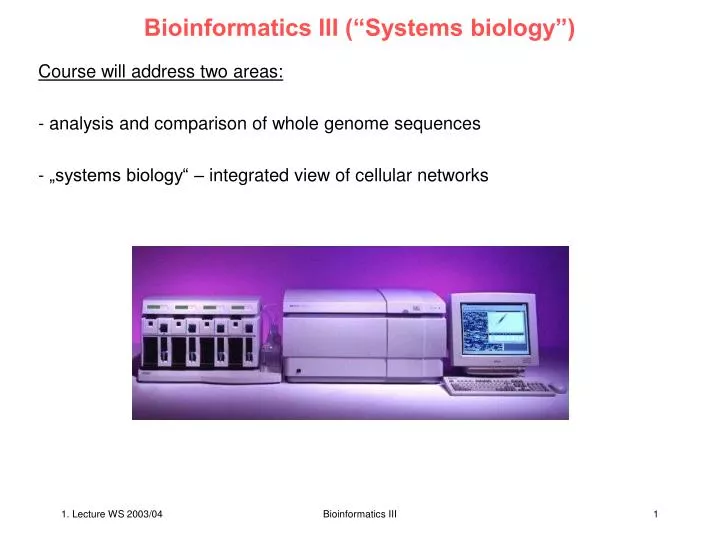
Bioinformatics III (“Systems biology”). Course will address two areas: analysis and comparison of whole genome sequences „systems biology“ – integrated view of cellular networks. Whole Genomes - Content. genome assembly gene finding genome alignment

E N D
Bioinformatics III (“Systems biology”) • Course will address two areas: • analysis and comparison of whole genome sequences • „systems biology“ – integrated view of cellular networks Bioinformatics III
Whole Genomes - Content genome assembly gene finding genome alignment whole genome comparison (prokaryotes, human mouse) genome rearrangements transcriptional regulation functional genomics phylogeny single nucleotide polymorphisms (SNPs) some topics were already covered in Bioinformatics 1 lecture by Prof. Lenhof Bioinformatics III
Cellular Networks - Content network topologies: random networks, scale free networks robustness of networks expression analysis metabolic networks, metabolic flow analysis linear systems, non-linear dynamics molecular systems biology: protein-protein interaction networks molecular machines ... Bioinformatics III
Literature • whole genome sequences • e.g. David Mount, Bioinformatics • Chapters 6, 8, 10 • system biology • mostly taken from original literature • Web-resources • - Institute of Systems Biology, Seattle, WA • http://www.systemsbiology.org/ • - The systems biology institute • http://www.systems-biology.org/ € 68 Bioinformatics III
assignments 12 weekly assignments planned Homeworks are handed out in the Tuesday lectures and are available on our webserver http://gepard.bioinformatik.uni-saarland.de on the same day. Solutions need to be returned until Tuesday of the following week 14.00 in room 1.05 Geb. 17.1, first floor, or handed in prior (!) to the lecture starting at 14.15. In case of illness please send E-mail to: kerstin.gronow-p@bioinformatik.uni-saarland.de and provide a medical certificate. Bioinformatics III
Schein = successful written exam The successful participation in the lecture course („Schein“) will be certified upon successful completion of the written exam on Feb. 18, 2004. Participation at the exam is open to those students who have received 50% of credit points for the 12 assignments. Unless published otherwise on the course website until Feb. 4, the exam will be based on all material covered in the lectures and in the assignments. In case of illness please send E-mail to: kerstin.gronow-p@bioinformatik.uni-saarland.de and provide a medical certificate. A „second and final chance“ exam may be offered at the beginning of April 2004 to those who failed the first exam and those who missed the first exam due to illness (medical certificate required). Bioinformatics III
tutors Prof. Dr. Volkhard Helms Sprechstunde: Tue 10-12. Geb. 17.1, room 1.06. Generally, I am also available after the lectures. Dr. Tihamer Geyer – assignments for network part Geb. 17.1, room 1.09. guest lecturers+tutors Bioinformatics III
Tree of Life Bacteria ArchaeaEukarya Euryarchaeota • Methanosarcina • Animals • Purple bacteria • Gram-positive • Halophiles • Methanobacterium • Fungi • Cyanobacteria • Methanococcus Chlamydiae Thermoplasma Thermococcus • Plants Slime molds Crenarchaeota Thermoproteus Pyrodictium • Flavobacteria Entamoebae Ciliates • Spirochetes • Deinococci • Green nonsulfur bacteria • Stramenophiles • Thermotogales • Trichomonads • Aquifex Microsporidia Diplomonads Bioinformatics III
Genomes A genome is the entire genomic material of any of these biological organism. We will review genome organization, known sequences, genome language, sequencing details etc. in the next lecture. Now that we have genome information from multiple organisms I see the following issues: 1 what biological questions do we ask? 2 what bioinformatics tools do we need to find the answers? 3 what are the answers? Bioinformatics III
Why mouse? 19 mouse chromosomes. Genetecists have anxiously awaited the recently published draft version of the Mouse genome? Why? Mouse as a close relative to humans is a unique lens through which we can view ourselves. As the leading mammalian system for genetic research over the past century it has provided a model for human physiology and disease. Comparative genomics makes it possible to discern biological features that would otherwise escape our notice. Nature 420, 520 (2002) Bioinformatics III
How do we compare genomes? Conservation of synteny between human and mouse. 558,000 highly conserved, reciprocally unique landmarks were detected within the mouse and human genomes, which can be joined into conserved syntenic segments and blocks. A typical 510-kb segment of mouse chromosome 12 that shares common ancestry with a 600-kb section of human chromosome 14 is shown. Blue lines connect the reciprocal unique matches in the two genomes. In general, the landmarks in the mouse genome are more closely spaced, reflecting the 14% smaller overall genome size. Nature 420, 520 (2002) Bioinformatics III
Genome rearrangements Segments and blocks >300 kb in size with conserved synteny in human are superimposed on the mouse genome. Each colour corresponds to a particular human chromosome. The 342 segments are separated from each other by thin, white lines within the 217 blocks of consistent colour. Genome rearrangments have functional implications (will be discussed later). Nature 420, 520 (2002) Bioinformatics III
Review: Pairwise sequence alignment • dynamic programming: Needleman-Wunsch, Smith Waterman • sequence alignments • substition matrices • significance of alignments • BLAST, algorithmn – parameters – output http://www.ncbi.nih.gov • This part of lecture taken from • O’Reilly book on “BLAST” by Korf, Yandell, Bedell • see also Bioinformatik I lecture by Prof. Lenhof • weeks 3 and 5 Bioinformatics III
Sequence alignment • When 2 or more sequences are present one would like • to detect quantitatively their similarities • discover equivalences of single sequence motifs • observe regularities of conservation and variability • deduce historical relationships • important goal: annotation of structural and functional properties assumption: sequence, structure, and function are inter-related. Bioinformatics III
Search in databases • Identify similarities between • a new test sequence, of • unknown and uncharacterized structure and function • and sequences in (public) sequence databaseswith known structure and function. • N.B. The similar regions can encompass the entire sequence or parts of it! • Local alignment global alignment Bioinformatics III
gap = Insertion oder Deletion Sequence Alignment The purpose of a sequence alignment is to arrange all those residues of a deliberate number of sequences beneath eachother that are derived from the same residue position in an ancestral gene or protein. J.Leunissen Bioinformatics III
Needleman-Wunsch Algorithm • general algorithm for sequence comparison • maximises a similarity score • maximum match = largest number of residues of one sequence that can be matched with another allowing for all possible deletions • finds the best GLOBAL alignment of any two sequences • NW involves an iterative matrix method of calculation all possible pairs of residues (bases or amino acids) – one from each sequence – are represented in a two-dimensional array all possible alignments (comparisons) are represented by pathways through this array. Three main steps 1 initialization 2 fill (induction) 3 trace-back Bioinformatics III
Needleman-Wunsch Algorithm: Initialization task: align words “COELACANTH” and “PELICAN” of length m=10 and n=7. Construct (m+1) (n+1) matrix. Assign values – m gap and – n gap to elements m and n of first row and first column. Here, gap = -1. Arrows of these fields point back to origin. Bioinformatics III
Needleman-Wunsch Algorithm: Fill Fill all matrix fields with scores and pointers using a simple operation that requires the scores from the diagonal, vertical, and horizontal neighboring cells. Compute • match score: value of upper left diagonal cell + score for a match (+1 or -1) • horizontal gap score: value of cell to the left + gap score (-1) • vertical gap score: value of cell to the top + gap score (-1) assign maximum of these 3 scores to cell. point arrow in direction of maximum score. max(-1, -2, -2) = -1 max(-2, -2, -3) = -2 (make arbitrary, consistent choice – e.g. always choose the diagonal over a gap. Bioinformatics III
Needleman-Wunsch Algorithm: Trace-back trace-back lets you recover the alignment from the matrix. start at the bottom-right corner and follow the arrows until you get to the beginning. COELACANTH -PELICAN-- Bioinformatics III
Smith-Waterman-Algorithm Smith-Waterman is a local alignment algorithm. SW is a very simple modification of Needleman-Wunsch. Only 3 changes: • edges of the matrix are initialized to 0 instead of increasing gap penalties. • maximum score is never less than 0. No pointer is recorded unless the score is greater than 0. • trace-back starts from highest score in matrix and ends at a score of 0. ELACAN ELICAN Bioinformatics III
Differences Needleman-WunschSmith-Waterman 1 Global alignments 1 Local alignments 2 requires alignment score for a pair 2 Residue alignment score may be of residues to be 0 positive or negative 3 no gap penalty required 3 requires a gap penalty to work efficiently more suited for alignment of eukaryotic sequences with exons and introns Bioinformatics III
Algorithmic complexity Dynamic programming methods such as Needleman-Wunsch and Smith-Waterman have O(mn) complexity in both time and memory. Variation: just use 2 rows at a time and don’t allocate the whole matrix. The alignment algorithm becomes O(n) in memory. Bioinformatics III
Scoring - or Substition Matrices • serve to better score the quality of sequence alignments. • for protein/protein comparison:a 20 x 20 matrix for the probabilities that certain amino acids are exchange others by random mutations • the exchange of amino acids of similar character (Ile, Leu) is more likely (receives higher score) than for exchanging amino acids of dissimilar character (e.g. Ile Asp) • scoring matrices are assumed to be symmetrical (exchange Ile Asp has the same probability as Asp Ile). Therefore they are triangular matrices. Bioinformatics III
Substitution matrices • Not all amino acids are similar • some can be replaced more easily than others • some mutations occur more frequently than others • some mutations are more long-lived than others • Mutations prefer certain exchanges • some amino acids have similar 3-letter codons • those residues are more replaced by random DNA mutation • Selection prefers certain exchanges • some amino acids have similar properties and structure (E.g. Trp cannot be inserted in the protein interior.) Bioinformatics III
PAM250 Matrix Bioinformatics III
Example Score The Score of an alignment is the sum of all invidual scores of the amino acid (base) pairs of the alignment. • Sequence 1: TCCPSIVARSN • Sequence 2: SCCPSISARNT • 1 12 12 6 2 5 -1 2 6 1 0=> Alignment Score = 46 Bioinformatics III
Dayhoff Matrix (1) • derived by M.O. Dayhoff who collected statistical data for probabilities of amino acid exchanges • data set for closely related protein sequences (> 85% identity). • advantage: these can be aligned to high certainty. • derive 20 x 20 matrix for probabilities of amino acid mutations from the observed frequency of exchanges • This matrix is called PAM 1. An evolutionary distance of 1 PAM (point accepted mutation) means that 1 point mutations occur per 100 residues. Or: both sequences are 99% identical. Bioinformatics III
Dayhoff Matrix (2) • Log odds Matrix: contains logarithms of PAM matrix entries. • Score of mutation i j • observed mutation rate i j= log( ) • expected mutation rate according to amino acid frequency • The probability of two independent mutational events is the product of the individual probabilities. • When using a log odds Matrix (i.e. using the logarithm of all values) one obtains the total alignment score as sum of the scores for every residue pair. Bioinformatics III
Dayhoff Matrix (3) • Derive Matrices for larger evolutionary distances by multiplying the PAM1 matrix with itself. • PAM250: • 2,5 mutations per residue • corresponds to 20% matches between two sequences, • i.e. mutations are observed at 80% of all residue positions. • This is the default matrix of most sequence analysis packages. Bioinformatics III
BLOSUM Matrix • limitation of Dayhoff-Matrix: the matrices based on the Dayhoff model of evolutionary rates are of limited value because the substitution rates were derived from sequence alignments of sequences that are more than 85% identical. • A different path was taken by S. Henikoff and J.G. Henikoff who used local multiple alignments of distantly related sequences. • Advantages: • larger data sets • multiple alignments are more robust Bioinformatics III
BLOSUM Matrix (2) • The BLOSUM matrices (BLOcks SUbstitution Matrix) are based on the BLOCKS database. • The BLOCKS database uses the concept of blocks (ungapped amino acid signatures) that are characteristic for protein families. • Derive probabilities of exchange for all amino acid pairs from the observed mutations inside the blocks. Convert into log odds BLOSUM matrix. • Different matrices are obtained by varying the lower requirement for the level of sequence identity. • e.g. the BLOSUM80 matrix is derived from blocks with > 80% identity. Bioinformatics III
Which matrix to use? • Close relationship (low PAM, high Blosum)Distant relationship (High PAM, low Blosum) • reasonable default parameters: PAM250, BLOSUM62
Gap penalties • Besides substitution matrices we need a method to score gaps • Which relevance do insertions or deletions have relative to substitutions? • distinguish introduction of gaps: • aaagaaa • aaa-aaa • from extension of gaps: • aaaggggaaa • aaa----aaa • different programs (CLUSTAL-W, BLAST, FASTA) recommend different default parameters which should be used as a first guess.
Significance of Alignments (1) • When is an alignment statistically significant?In other words: • How different is the obtained score of an alignment from scores that would result from alignments of the test sequence with random sequences? • Or: • What is the probability that an alignment of this score occured randomly? Bioinformatics III
Significance of Alignments (2) • size of database = 20 x 106 letters • Peptide #hits • A 1 x 10⁶ (if equally distributed) • AP 50000 • IAP 2500 • LIAP 125 • WLIAP 6 • KWLIAP 0,3 • KWLIAPY 0,015 Bioinformatics III
BLAST – Basic Local Alignment Search Tool • finds the highest-scored local optimal alignment of a test sequence with all sequences of a database. • Very fast algorithm. Ca. 50 times faster than dynamical programming. • because BLAST uses pre-indexed database, BLAST can be used to search very large databases. • is sufficiently sensitive and selective for most purposes. • Is robust – default parameters usually work fine. Bioinformatics III
test sequence L N K C K T P Q G Q R L V N Q P Q G 18 word P E G 15 related P R G 14 words P K G 14 P N G 13 P M G 13 P Q A 12 below cut-off(T=13) P Q N 12etc. BLAST Algorithm, Step 1 • For given word of length w (usually 3 for proteins) and for a given scoring matrix • construct list of all words (w-mers) which get score > T if compared to w-mer of input sequence. P D G 13 Bioinformatics III
P Q G 18 P E G 15 PMG P R G 14 Database P K G 14 P N G 13 P D G 13 P M G 13 BLAST Algorithm, Step 2 • each related word points to positions in data base (hit list). Bioinformatics III
BLAST Algorithm, Step 3 • Program tries to extend suitable segments (seeds) in both directions by adding pairs of residues. • Residues are added until score sinks below cut-off. Bioinformatics III
different BLAST algorithms • BLASTN – compares nucleotide sequence against nucleotide database • BLASTP – compares protein sequence against protein database • BLASTX – compares nucleotide sequences translated in all 6 open reading frames against protein sequence database • TBLASTN • TBLASTX Bioinformatics III
BLAST Output (1) Small probability shows that hit is likely not random Bioinformatics III
Significance of BLAST alignment P-value (probability) • probability that alignment score could result from alignment of random sequences • the closer P equals 0, the higher is certainty that a hit is a true hit (homologous sequence) E-value (expectation value) • E = P * number of sequences in database • E is the number of alignments of a particular score that can be expected to occur randomly in a sequence database of this size • if e.g. E=10, one expects 10 random hits with the same score. Such an alignment is not significant. Use appropriate threshold in BLAST. Bioinformatics III
Rough guide • P-value (probability) – A. M. Lesk • P 10-100 sequences are identical • 10-100 < P < 10-50 sequences are almost identical, e.g. alleles or SNPs • 10-50 < P < 10-10 closely related sequences, homology is certain • 10-10 < P < 10-1 sequences are usually distantly related • P > 10-1 similarity probably not significant • E-value (expectation value) • E 0,02 sequences probably homologous • 0,02 < E < 1 Homology possible • E 1 good agreement most likely random. Bioinformatics III
Rough guide Level of sequence identity with optimal alignment • > 45% proteins have very similar structure • and most likely the same function • > 25% proteins probably possess similar fold • 18 – 25% Twilight-Zone - assuming homology is tempting • below alignment has little significance Bioinformatics III
Twilight-Zone (1) • myoglobin from whale and Leghemoglobin of lupins are 15% identical with optimal alignment • both have very similar tertiary structure. • both contain heme group and bind oxygen • they are remotely related, though homologous proteins Left: Whale Mb Right: Leg Hb www.rcsb.org Bioinformatics III
Twilight-Zone (2) • the N- and C-terminal halfs of thiosulfate-sulfate-transferase have 11% sequence identity. • Because they belong to the same protein assumption that they resulted from gene duplication and divergent evolution. • Indeed both 3D structures show large similarity. 2ORA Rhodanese www.rcsb.org Bioinformatics III
Twilight-Zone (3) • serine proteases chymotrypsin and subtilisin • have 12% identity with optimal alignment • both have same function, same catalytic triad of 3 amino acids (Ser – His – Asp) • However, the two folds are completely different and the proteins are not related. Example for convergent evolution. Left: 1AB9- Bovine Chymo Trypsin Right: 1GCI Bacillus Lentus Subtilisin www.rcsb.org Bioinformatics III
Summary Pairwise alignment of sequences is routine but not trivial. Dynamic programming guarantees finding the alignment with optimal score (Smith-Waterman, Needleman-Wunsch). Much faster but reliable tools are: FASTA, (PSI) BLAST Deeper functional insight into sequences and relationships from multiple sequence alignments (see lecture on phylogenies). Bioinformatics III
Growth of Proteomic Data vs. Sequence Data Bioinformatics III