Explicit Convective Forecast with WRF-ARW for the Warm Seasons in the United States

1. Explicit Convective Forecast with WRF-ARW for the Warm Seasons in the United States MPO 563 Convective and Mesoscale Meteorology I-Kuan Hu Caution! Not even a single WRF simulation has been run in this project!

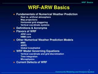
2. Challenges for Numerical Weather Prediction • Prediction of convective weather (meso- and smaller scales) is a major contributor to poor warm season quantitative precipitation forecasting. Errors could be attributed to… (Skamarock et al. 2005 [v.2] & 2008 [v.3]) • Initial conditions (ICs)/lateral boundary conditionsFrom observation, coarser simulation of other NWP models, or both. Data assimilation plays an important role in this part. • Physical setsIn WRF: cumulus parameterization, microphysics, PBL, land-surface model, surface layer, and atmospheric radiation. • Model configuration

3. Cumulus Parameterization • “Parameterization”Designed to represent the effects of the smaller-scale processes in terms of the large-scale state.A Cumulus (or cloud, or convective) parameterization represents the cloud processes in terms of the large-scale atmospheric states (ex: temperature, moisture, low-level convergence). • ChallengesOne major source of the uncertainty in the numerical models. Uncertainties could be attributed to various types of cloud, microphysics, entrainment/detrainment, turbulence, …Randall et al. (2003): “It is ironic that we cannot represent the effects of the small-scale processes by making direct use of the well-known equations, in which we have the most confidence, that govern them.” “… or can we ?”

4. Explicit Convective forecast • “Explicit convection” - no cumulus parameterization!Also “convection-allowing”, “convection-permitting”, or “cloud-resolving” forecasts, which provide a more accurate depiction of the physics of convective systems • Horizontal resolution mattersWeisman et al. (1997): 4-km grid spacing is adequate to represent the basic structure, mass and momentum transport of idealized MCSs. • WRF-ARW 36-h real-time forecasts The Bow-Echo and Mesoscale Convective Vortex Experiment (2003), WRF Real-Time Catalog (2004-08), Hazard Weather Testbed Spring Forecasting Experiment (2008-12).

5. In this talk, we will… • Use two cases from 04-08 WRF real time catalog to compare MCSs in the observations, explicit convective forecasts, and coarser-resolution simulations using convective parameterizations. • Learn how the state-of-the-art data assimilationcan improve the ICs for explicit convective forecasts.

6. Case 1: Squall Line at 5 June 2005 NOWRAD 18 UTC 04 June – 12 UTC 05 June

7. Case 1: Squall Line at 5 June 2005 NOWRAD 18 UTC 04 June – 12 UTC 05 June (Fig. 10 in Weisman et al., 2008; http://catalog.eol.ucar.edu/wrf-2005/)

8. Case 1: Squall Line at 5 June 2005 NOWRAD18 UTC 04 June – 12 UTC 05 June ARW 4km initialized 00 UTC 04 June 18-36 h Forecasts

9. Case 1: Squall Line at 5 June 2005 NOWRAD18 UTC 04 June – 12 UTC 05 June ARW 4km initialized 00 UTC 04 June 18-36 h Forecasts (Fig. 10 in Weisman et al., 2008; http://catalog.eol.ucar.edu/wrf-2005/)

10. Case 1: Squall Line at 5 June 2005 NAM 12 km 24-30 h ARW 12 km 24-30 h ARW 4 km 24-30 h ST4 00-06 UTC 05 June (Fig. 11 in Weisman et al., 2008)

11. Case 2: MCV at 1 June 2007 NOWRAD 18 UTC 31 May – 12 UTC 01 June

12. Case 2: MCV at 1 June 2007 NOWRAD 18 UTC 31 May – 12 UTC 01 June (Clark et al., 2010; http://catalog.eol.ucar.edu/wrf_2007/)

13. Case 2: MCV at 1 June 2007 NOWRAD18 UTC 04 June – 12 UTC 05 June ARW 4km initialized 00 UTC 31 May 18-36 h Forecasts (Clark et al., 2010; http://catalog.eol.ucar.edu/wrf_2007/)

14. Case 2: MCV at 1 June 2007 NOWRAD18 UTC 04 June – 12 UTC 05 June ARW 4km initialized 00 UTC 31 May18-36 h Forecasts (Clark et al., 2010; http://catalog.eol.ucar.edu/wrf_2007/)

15. Daily Variation Numbers of MCSs (13 May – 9 July 2003) Total # of MCSsObs:142 4-km WRF: 109 10-km WRF:99 Correlation4-km WRF & Obs:0.57 10-km WRF & Obs: 0.35 (Fig. 4 in Done et al., 2004)

16. Data Assimilation • Data assimilation for the ICsThe process by which observations are incorporated into an estimate (“background” guess) of the initial state over a domain, a period of time, and for all variables in a model’s simulation. • Data Assimilation Research TestbedAn open-source community developed and maintained at NCAR. Provides toolkit that combined with continuous data assimilation and the ensemble Kalman filter for WRF-ARW’s ICs. Also easily assimilate some new data sets such as GPS radio occultation. no GPS radio occultation with GPS radio occultation (Fig. 4 in Anderson et al. 2009; Romine et al. 2013)

17. Data Assimilation Observation (batches) 00 UTC 06 UTC 12 UTC • Intermittent DAObservations are assimilated in batches at a given analysis time (determined by cycling interval). • Continuous DA (more popular now)Very small cycling interval, permits forecast to be launched at any desired time from the DA system.The model must always be running (EXPENSIVE!). Data Assimilation Ana/Init Ana/Init Ana/Init Background Background Background Forecasts

18. Data Assimilation • The Kalman filterA least square (variance) estimate:: analysis, : forecast background, : observations., : variance (uncertainty) of and from the true field (unknown), mostly estimated as a specific distribution (probability density function). • However, real atmosphere is multidimensional→ and need to be expressed as covariance matrices(HUGE amount of data). → Not common in weather forecasting models. • The Ensemble Kalman filter (more popular now) estimated from a finite ensemble of forecasts can represent the nearly same error statistic as a full covariance matrix.

19. Summary • What is explicit convective forecast?Fully explicit forecast with 4-km or smaller horizontal grid spacing to avoid uncertainties inherent with convective parameterization schemes used in coarser-resolution models. • AdvantagesForecasts realistically represent the structure and evolution of mesoscale convective phenomena (squall lines, mesoscale convective vortices and bow echoes); also provide a more accurate depiction of the physics of convective systems. • LimitsNo obvious improvements in forecasting the location, timing and relative intensities of convective systems. It could be due to the sensitivities to other physical configurations, or the uncertainties of the ICs/lateral conditions. However, the latter one could be improved by combining the model with the state-of-the-art data assimilation.

20. References • Weisman et al., 1997: The resolution dependence of explicitly modeled convective systems. Mon. Wea. Rev., 125, 527-548. • Randall et al., 2003: Breaking the Cloud Parameterization Deadlock. Bull. Amer. Meteor. Soc., 84, 1547-1564. • Done et al., 2004: The next generation of NWP: Explicit forecasts of convection using the Weather Research and Forecast (WRF) model. Atmos. Sci. Lett., 5, 110-117. • Weisman et al., 2008: Experiences with 0-36-h explicit convective forecasts with the WRF-ARW Model. Wea. Forecasting,23, 407-437. • Skamarock et al., 2008: A description of Advanced Research WRF version 3. NCAR Tech. Note NCAR/TN-475+STR, 125 pp. • Anderson et al., 2009: The Data Assimilation Research Testbed: A Community Facility. Bull. Amer. Meteor. Soc.,90, 1283-1296. • Clark et al., 2010: Convection-Allowing and Convection-Parameterizing Ensemble Forecasts of a Mesoscale Convective Vortex and Associated Severe Weather Environment. Wea. Forecasting.,25, 1052-1081. • Romine et al., 2013: Model Bias in a Continuously Cycled Assimilation System and Its Influence on Convection-Permitting Forecasts. Mon. Wea. Rev.,141, 1263-1284. • WRF Real-Time Catalog 04-08:http://catalog.eol.ucar.edu/wrf-2004 (-2005, -2006, _2007, _2008)

21. Thank you!Questions? Or time for 2-day’s forecast? NCEP’s Model Analysis & Guidance