Download
1 / 31
320 likes | 461 Views
Walk&Sketch : Create Floor Plans with an RGB-D Camera. Ying Zhang 1,3 Chuanjiang Luo 2 J uan Liu 1. 1 Palo Alto Research Center 2 Ohio State University 3 Current Affiliation: Google Inc. ACM UbiComp12: Sep. 5 – Sep. 8 , 2012.

E N D
Walk&Sketch: Create Floor Plans with an RGB-D Camera Ying Zhang1,3 Chuanjiang Luo2 Juan Liu1 1 Palo Alto Research Center 2 Ohio State University 3 Current Affiliation: Google Inc. ACM UbiComp12: Sep. 5 – Sep. 8, 2012
Motivation: Cheap and Efficient Floor Plan Generation for Existing Buildings • Problem: • Existing old buildings do not have updated floor plans • Creating floor plans for an existing space can be expensive • Solution: • RGB-D cameras are cheap and widely available • 3D models have been generated in real time from existing research • Challenges: • Noise/ambiguity handling • 2D Map extracting
Prototype and Concept of Operations (CONOP) • Prototype: Backpack, that holds • PC Laptop with USB ports, connected to • Kinect with a battery pack • iPad (handheld) optional • CONOP: • Hold PC laptop or iPad at hand, start mapping from scratch or from an initial position on a map • Walk in normal strolling speed, keeping in the middle of a hallway or within ~2-3 meters to the wall • Create sketch floor maps of the explored area on the handheld user interface
System Architecture • 6D Camera Trajectory Computation, Output • Global Camera Trajectories • Local 3D Point Clouds of Key Frames • 2D Polyline Map Extraction, Output • Global 2D Map by a set of Polylines • Explored Area Coverage, Output • Explored Area by Overlapping Polygons
Motivation, Prototype and System Architecture • Camera Trajectory Computation • Preprocessing • Local matching between neighboring frames • Global matching between key frames • 2D Polyline Map Generation • Segmentation • Rectification • Map merging • Explored Area Computation • Future Research
Camera Trajectory Computation: Preprocessing Local Matching
Local Matching • Aligns each of two adjacent frames • Output: • 6D camera pose between adjacent frames • 3*3 covariance error matrix for the translation part
Local Matching SIFT of frame1 Modified RANSAC ICP SIFT of frame2
Uncertainty for local matching • Calculate Covariance Matrices for Translational Error: • Close Loop by Error Distribution: • Angular: evenly distribute among the key frames in the loop • Translational: distribute according to covariance matrices of the key frames in the loop
Global matching • Loop Detection: • A loop is detected if the new key frame matches any of the previous key frames Frame i Frame i+2 Frame k Frame i+1
Motivation, Prototype and System Architecture • Camera Trajectory Computation • Preprocessing • Local matching between neighboring frames • Global matching between key frames • 2D Polyline Map Computation • Segmentation • Rectification • Map merging • Explored Area Computation • Future Research
Algorithm Flowchart (2D floor map) 3D Transforms Point Clouds Line Segmentation SketchTo Polyline Rectification Polylines Sketch map Merging Sketch Polyline map
Line Segmentation • Get a 2D slice at certain fixed height: • We choose a height above common types of furniture to get wall outlines better. • Order points in the 2D slice along the camera viewing angle: • This allows more efficient line segmentation (without optimization). • Order is preserved during motion. • Two phases of line segmentation: • Linearization: move along the ordered points to form a line until it breaks • Clustering: merge two segments if they are almost align with each other break α new segment extend sin(α)>K min Ai>T Linearization Clustering
Rectification • Assumption: wall segments are rectilinear • First few frames: Compute wall orientation (with modulo 90 degrees) using a statistical approach: • We set the camera to face the rectilinear walls initially • We choose the average direction modulo 90 degrees [-45o, 45o] as the wall directions if its standard deviation is small enough • Following frames: Compute wall orientation of the current frame, if • it is significantly different from the initial wall orientation, or • its standard deviation is large Ignore the frame, otherwise • Rectify the frame to the wall orientation so that walls are aligned
Sketch Merging from Sketch1 to Sketch2 • Line segments are directional • For each line in Sketch1, there is a line of the same direction in Sketch2 that overlaps with, when: • The distance between them is < maxD (0.5 meters) • They either cross each other or the gap between them is < maxD • If two lines overlap, a merged line is obtained by: (x22, y) (x12, y1) (x11, y1) (x11, y) (x22, y2) (x21, y2)
Motivation, Prototype and System Architecture • Camera Trajectory Computation • Preprocessing • Local matching between neighboring frames • Global matching between key frames • 2D Polyline Map Extraction • Segmentation • Rectification • Map merging • Explored Area Computation • Future Research
Explored Area Computation • Input • Sketch map: a set of lines • Position and orientation of the sensor: 2D <x,y,α> or 3D <x,y,z,α,β,γ> • Viewing polygon of the sensor (next slide) • Output • Viewing polygon of each frame after clipping of walls • Explored area to be the union of all viewing polygons
Examples of the Viewing Polygons of Sensors p5 p3 p4 p1 p1 p2 p2 p3 Camera (90o View) Laser (270o View) p5 p6 p1 p4 p2 p3
Property of a Viewing Polygon • There is an origin where the sensor is located • There is only one intersection from the center to any point on the boundary lines of the viewing polygon o o
Simple Viewing Polygon Clipping Cases o • Both ends in range • One end in and one end out • Both ends out of range, but the line cuts the polygon o o
Complex (Concave) Polygon Clippings 1 2 Each internal point has a correspondent boundary point Create a new polygon by computing and ordering all internal, boundary and intersection points 3
Polygon Clip (X or Y) • Given sensor location and orientation, and the initial viewing polygon in sensor’s frame, compute the viewing polygon in the reference frame, • For each line in the set which is in the range of the polygon, do a subtraction of the polygon
Conclusions and Future Work • A prototype system to create floor plan • It is implemented in Matlab • Good accuracy • Future Work: • Implement a real-time prototype using a gaming laptop with GPU for image processing • Add feature detection for windows, doors and common furniture to annotate the map automatically